Autoregressive models provide a simple yet useful framework to predict future values based on past observations. The forecasting model uses past values (\(Y_{t-1}, Y_{t-2}, Y_{t-3}, \dots\)) to forecast \(Y_{t}\).
5.1 AR
To predict the future, a natural place to start is the immediate past. The AR(1) model frames this simplest case, where only the immediately previous observation influences the current one:
\[
Y_t = \phi_0 +\phi_1 Y_{t-1}+ \varepsilon_t
\]
where:
\[\begin{align}
Y_t: & \ \text{the value of $Y$ at time} \ t \\
\phi_0: & \ \text{constant term} \\
\phi_1: & \ \text{autoregressive coefficient} \\
\varepsilon_t: & \ \text{white noise error}
\end{align}\]
The coefficients \(\phi_0\) and \(\phi_1\) can be estimated using OLS regression. No causal interpretation should be assumed.
NoteExample
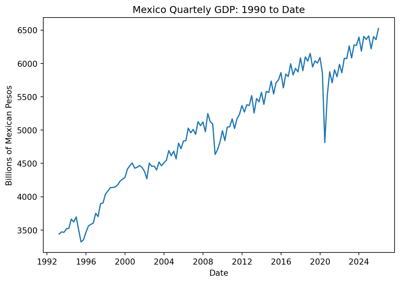
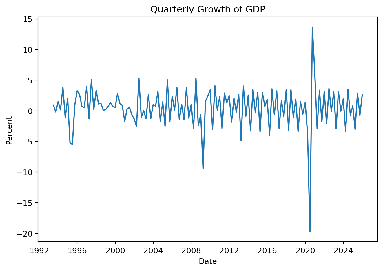
Adjust Autoregressive models to GDP data for Mexico. Stationarity is required, the idea is that a process whose behavior is stable over time is also predictable.
Show code
import pandas as pdimport numpy as npimport matplotlib.pyplot as pltimport statsmodels.api as smfrom datetime import datetimeimport yfinance as yffrom pandas_datareader import data as pdrfrom statsmodels.tsa.stattools import adfuller, kpssfrom statsmodels.stats.diagnostic import acorr_ljungboxfrom statsmodels.tsa.ar_model import AutoRegimport plotly.graph_objects as gofrom scipy.stats import norm
Show code
GDP = pdr.DataReader('NGDPRNSAXDCMXQ', 'fred', start='1993Q1', end ='2026Q1')GDP = GDP.rename(columns={'NGDPRNSAXDCMXQ': 'Values'})GDP = GDP.reset_index()GDP = GDP.rename(columns={'DATE': 'Date'})GDP['Date'] = pd.to_datetime(GDP['Date'], dayfirst=True) + pd.offsets.QuarterEnd(0)GDP.set_index(pd.PeriodIndex(GDP['Date'], freq='Q'), inplace=True)GDP['Values'] = GDP['Values']/1000# Mil millones
plt.figure(figsize=(7, 5))plt.plot(GDP['Date'], GDP['Values'])plt.xlabel('Date')plt.ylabel('Billions of Mexican Pesos')plt.title('Mexico Quartely GDP: 1990 to Date')plt.tight_layout()# plt.grid(True)plt.show()
Clearly the series is not stationary. Formally, implement the tests:
/var/folders/wl/12fdw3c55777609gp0_kvdrh0000gn/T/ipykernel_69787/1519198186.py:2: InterpolationWarning:

The test statistic is outside of the range of p-values available in the
look-up table. The actual p-value is smaller than the p-value returned.
/var/folders/wl/12fdw3c55777609gp0_kvdrh0000gn/T/ipykernel_69787/3253650088.py:2: InterpolationWarning:

The test statistic is outside of the range of p-values available in the
look-up table. The actual p-value is greater than the p-value returned.
Tests suggest the time series of GDP growth is stationary.
The adjusted r-squared increases only slightly relative to the AR(1) model and the second lag is not statistically significant. Most of the variation in next-quarter’s GDP growth remains unforecasted. Can we do better?
5.1.3 Forecast Error and Confidence intervals
5.1.3.1 Root Mean Squared Forecast Error (RMSFE)
Because the forecasting model is estimated using historical data available at the time the model is estimated, a forecast is an out-of-sample prediction of the future. Forecasts can either be one-step ahead or multiple steps ahead, for instance:
\[
Y_{T+1|T}
\] represents the forecast of \(Y\) at date \(T+1\) based on data through date \(T\). This implies a forecast error:
\[
Y_{T+1}-\hat{Y}_{T+1|T}
\]
The accuracy of a model’s predictions can be measured with the Mean Squared Forecast Error (MSFE). It quantifies the average difference between the actual (observed) values and the predicted values produced by the model. More formally, it is the expected value of the square of the forecast error, when the forecast is made for an observation not used to estimate the forecasting model (i.e., for an observation in the future).
\[
MSFE = E\big[Y_{T+1}-\hat{Y}_{T+1|T}\big]^2
\]
Using the square of the error penalizes large forecast error much more heavily than small ones. A small error might not matter, but a very large error could call into question the entire forecasting exercise.
The Root Mean Squared Forescast Error (RMSFE) derives from the MSE, but has the same units as the series being forecast so its magnitude is more easily interpreted, this is:
\[
RMSFE = \sqrt{E[Y_{T+1}-\hat{Y}_{T+1|T}]^2}
\]
The RMSFE is like the standard deviation, except that it explicitly focuses on the forecast error using estimated coefficients. It can be understood a measure of the magnitude of a typical forecasting “mistake”.
The method we employ to estimate the MSFE is based on simulating how the forecasting model would have done, had we been using it in real time.
– Choose a date \(P\) for the start of a pseudo out-of-sample (POOS), for example \(P = 0.8T\).
– Re-estimate your model every period, \(s = P−1,…,T−1\)
– Compute the forecast error: \(Y_{s+1}-\hat{Y}_{s+1|s}\)
– Plug this forecast error into the equation: \(MSFE_{POOS}=\frac{1}{P} \sum_{s=T-P+1}[Y_{s+1}-\hat{Y}_{s+1|s}]^2\)
Return to the example of predicting the next quarter GDP growth to approximate the forecast error. Start a pseudo out-of-sample (POOS) by splitting the sample into ‘train’ and ‘test’ sub-samples:
y_roll = GDP['y'] T =len(y_roll)P =int(0.8* T) # 80% train
Fit the AR(1) model recursively and use it to forecast one step ahead
forecasts = []actuals = []# Rolling POOS forecastfor s inrange(P, T -1):# Fit model on data up to time s model = AutoReg(y_roll[:s+1], lags=1, old_names=False).fit()# Forecast y_{s+1} y_pred = model.predict(start=s+1, end=s+1).iloc[0] forecasts.append(y_pred) actuals.append(y_roll.iloc[s+1])
The RMSFE can be used as an estimate of the forecast error variance, which feeds directly into confidence intervals. A \((1-\alpha)\) forecast interval can be constructed as
The \(Z-value\) is found using the inverse of the CDF from the normal distribution. This assumes the innovation \(\varepsilon_t\) in the AR model is normally distributed.
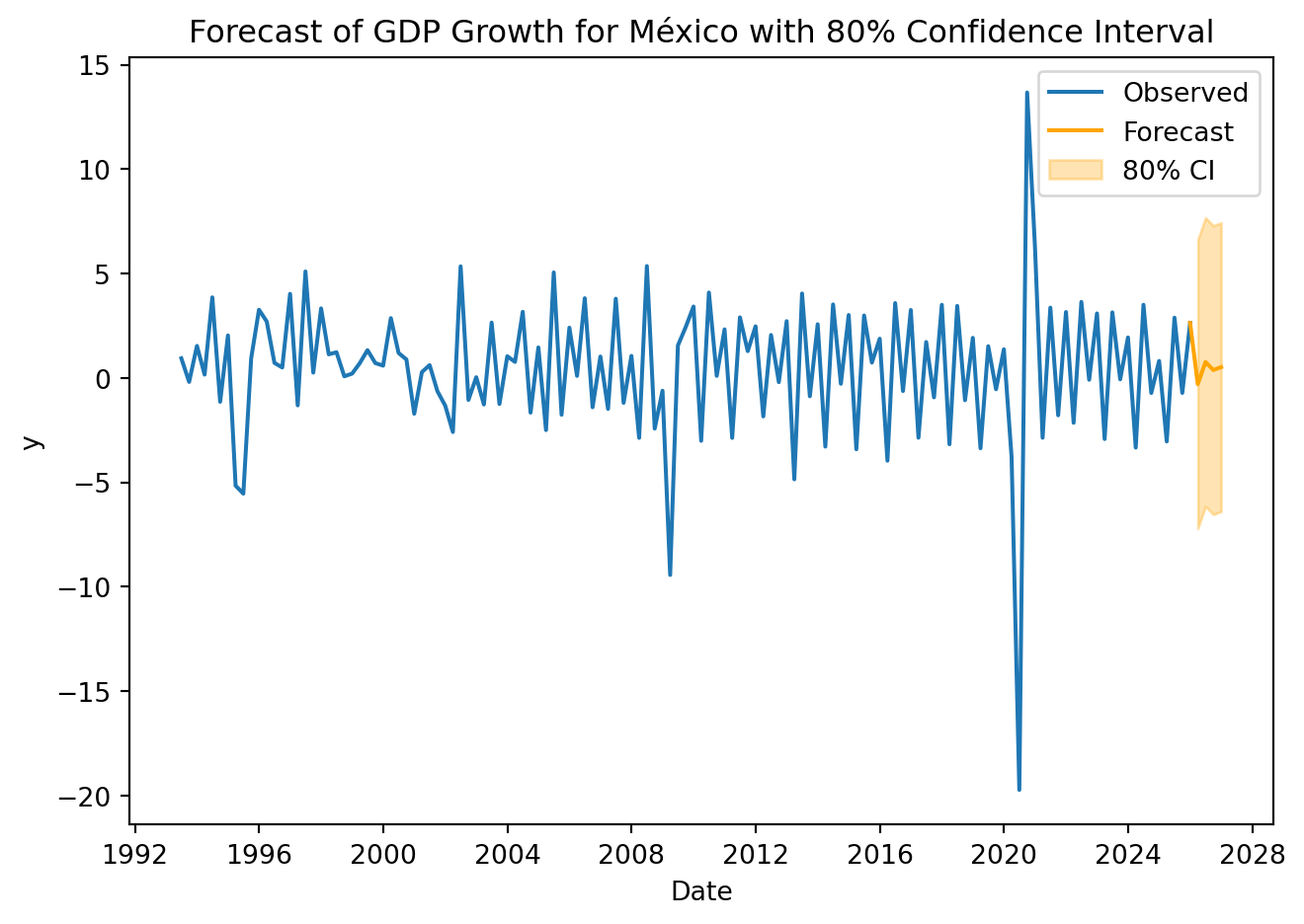
Continuing with the example:
Recall the forecast of GDP growth using an AR(1) model is:
from scipy.stats import norm# For a 80% confidence intervalalpha =0.20z = norm.ppf(1-alpha/2)ci_lower = forecast_T1 - z * rmsfeci_upper = forecast_T1 + z * rmsfeprint(f"2025 Q4 Forecast: {forecast_T1:.4f}")print(f"80% CI (based on RMSFE): [{ci_lower:.4f}, {ci_upper:.4f}]")
2025 Q4 Forecast: -0.2975
80% CI (based on RMSFE): [-7.2129, 6.6180]
Forecasting the next 4 quarters:
forecast_horizon =4f_values = []current_y = last_yfor _ inrange(forecast_horizon): next_y = final_model.params['const'] + final_model.params['y.L1'] * current_y f_values.append(next_y) current_y = next_yci_upper = [f + z * rmsfe for f in f_values]ci_lower = [f - z * rmsfe for f in f_values]
Show code
GDP['Date'] = pd.to_datetime(GDP['Date'])last_date = GDP['Date'].iloc[-1]forecast_dates = pd.date_range(start=last_date + pd.offsets.QuarterEnd(), periods=4, freq='QE')extended_dates = [GDP['Date'].iloc[-1]] +list(forecast_dates)extended_values = [GDP['y'].iloc[-1]] + f_values# Plotplt.figure(figsize=(7, 5))plt.plot(GDP['Date'], GDP['y'], label='Observed')plt.plot(extended_dates, extended_values, label='Forecast', color='orange')plt.fill_between(forecast_dates, ci_lower, ci_upper, color='orange', alpha=0.3, label='80% CI')plt.title('Forecast of GDP Growth for México with 80% Confidence Interval')plt.xlabel('Date')plt.ylabel('y')plt.legend()plt.tight_layout()plt.show()
While we ony employ AR(1) and AR(2) models in this example, the order of the autoregression can be extended. An autorregresive model of order p, AR(p), is written as:
where \(\varepsilon_t\) is white noise and restrictions on the values of \(\phi\) apply due to stationarity requirements.
NotePractice
In this activity, you will estimate an AR(1) model to forecast U.S. inflation (FRED code: CPIAUCSL). Using monthly data from 2010 to 2026, forecast three months ahead, and construct 90% forecast confidence intervals using an out-of-sample measure of forecast accuracy.
Forecasting U.S. inflation is highly relevant for Mexico. The United States is Mexico’s largest trading partner, and inflation dynamics in the U.S. influence Mexico’s macroeconomic indicators including export demand, exchange rate movements, and monetary policy decisions by Banco de México.
Because inflation in more advanced economies tends to exhibit persistence, short-term dynamics are often reasonably approximated by an AR(1) process.
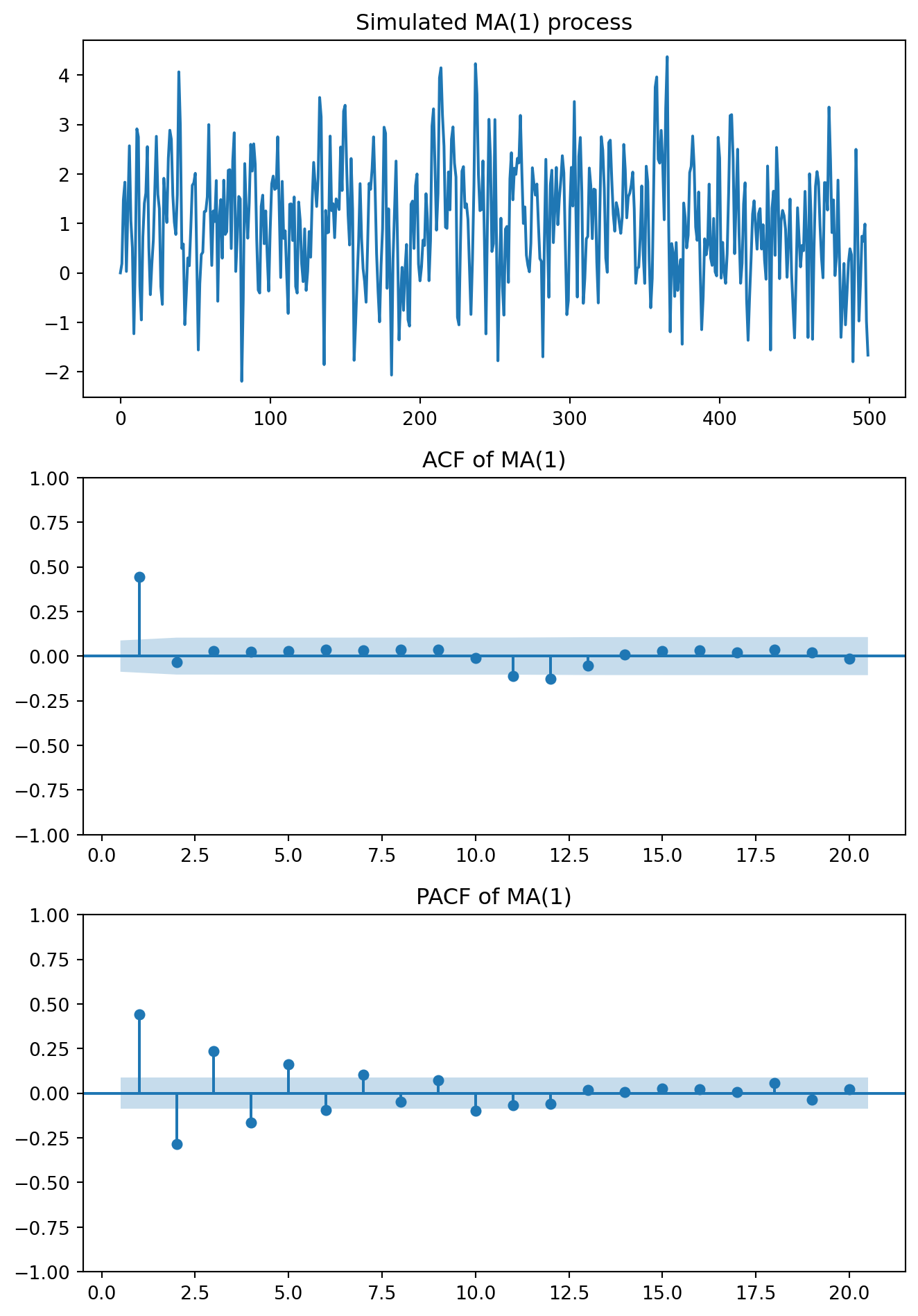
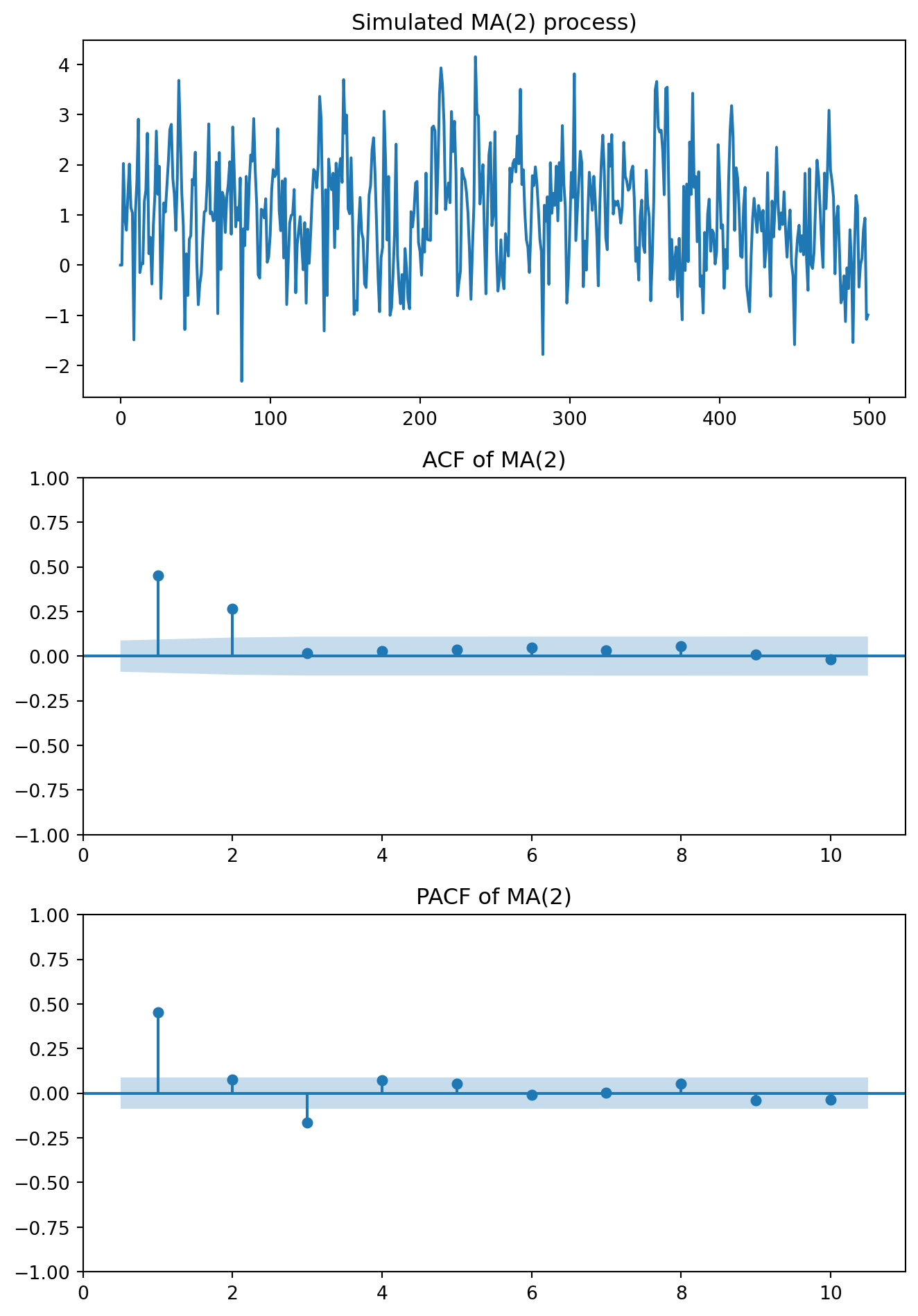
5.2 MA
So far, we have assumed that persistence in the series comes from past values of the variable itself, but persistence might come from past shocks. This possibility leads us to Moving Average (MA) models.
If an MA model is invertible, then the invertible \(MA(q)\) process can be written as an \(AR(\infty)\). For MA(q), invertibility is ensured if the roots of the MA polynomial \(1+\theta_1z + \cdots + \theta_qz^q=0\) lie outside the unit circle.
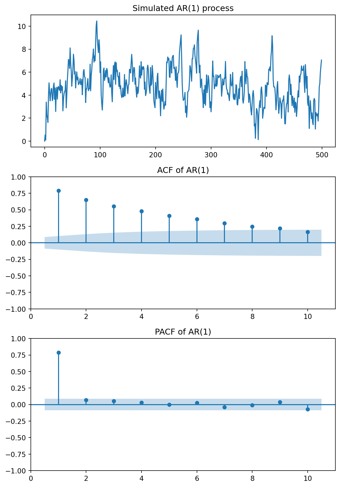
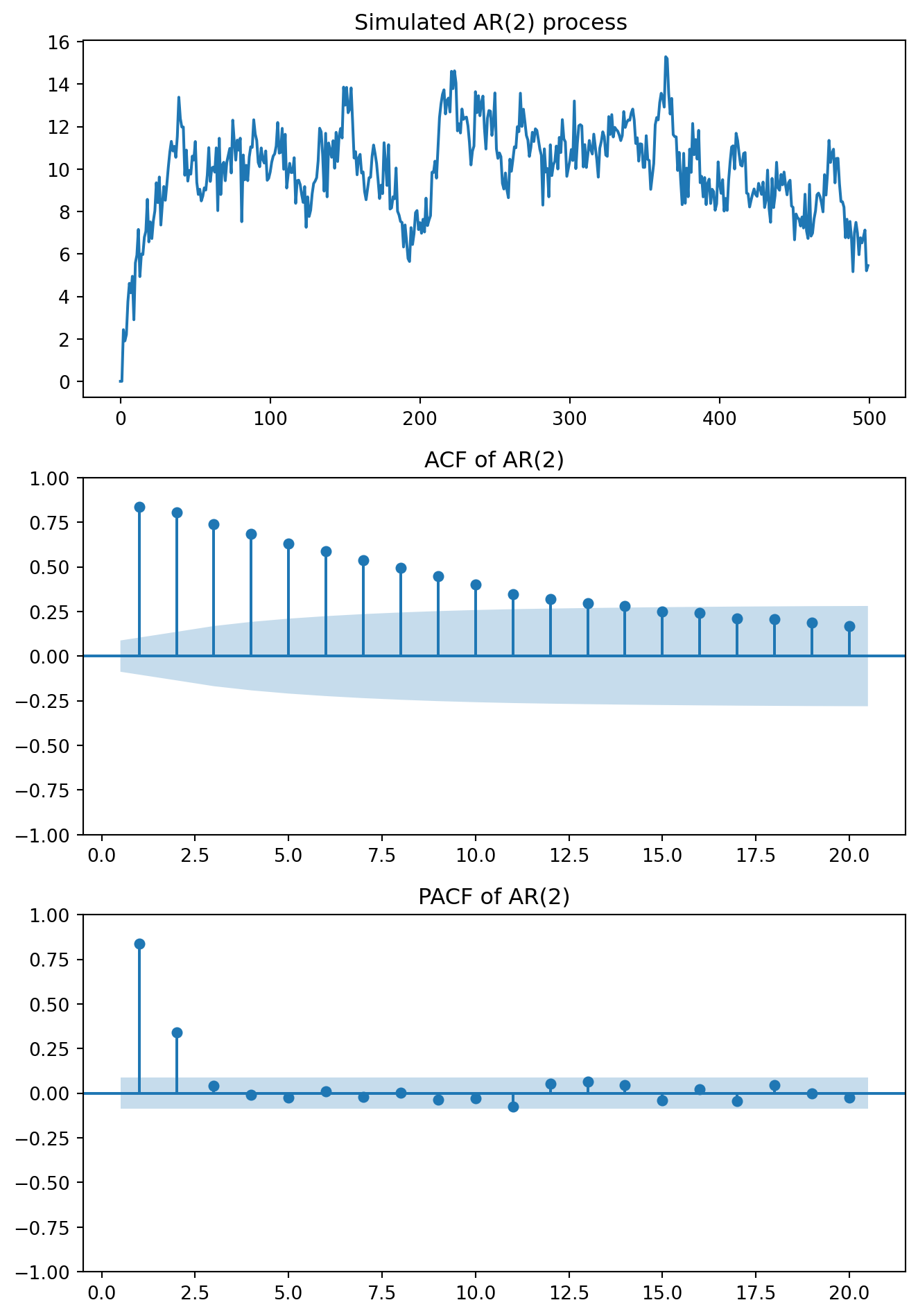
phi1 =0.5phi2 =0.4np.random.seed(1234)eps = np.random.normal(loc=0.0, scale=1.0, size=T)y_ar2 = np.zeros(T)# Start at t = 2 so that y_{t-1} and y_{t-2} existfor t inrange(2, T): y_ar2[t] = mu + phi1 * y_ar2[t-1] + phi2 * y_ar2[t-2] + eps[t]fig, axes = plt.subplots(3, 1, figsize=(7, 10))axes[0].plot(y_ar2)axes[0].set_title("Simulated AR(2) process ")plot_acf(y_ar2, lags=20, ax=axes[1], zero =False)axes[1].set_title("ACF of AR(2)")plot_pacf(y_ar2, lags=20, ax=axes[2], zero =False)axes[2].set_title("PACF of AR(2)")plt.tight_layout()plt.show()
ACF: decays gradually (oscillates if \(\phi_2\) is negative)
PACF: strong at lags 1 and 2, near zero after lag 2.
Diagnostic:
For MA(q):
– ACF: cuts off after lag q
– PACF: tails off gradually
For AR(p):
– PACF: cuts off after lag p
– ACF: tails off gradually
5.3 ARMA/ARIMA
The combination of an autoregression (AR) and a moving average (MA) model, is an ARMA model. ARMA is an acronym for AutoRegressive Moving Average. An ARMA(p,q) process, is written as:
ARIMA is the acronym for AutoRegressive Integrated Moving Average. An ARIMA(p,d,q) process, is written as:
\[
Y'_{t} = \mu + \phi_{1}Y'_{t-1} + \phi_{2}Y'_{t-2} + \dots + \phi_{p}Y'_{t-p} + \varepsilon_t + \theta_{1}\varepsilon_{t-1} + \theta_{2}\varepsilon_{t-2} + \dots + \theta_{q}\varepsilon_{t-q}
\] where \(Y'\) is the differenced series.
where:
p:
Order of the autoregressive component
q:
Order of the moving average component
d:
Degree of differencing
Information Criteria
ACF and PACF will not help to distinguish ARIMA models when \(p,q>0\). In practice, several alternative specifications of ARIMA models are usually possible. In these situations, we need a way to compare competing models and select the one that better balances good fit with parsimony.
For this purpose we use information criteria. Two commonly used metrics are the Akaike Information Criterion (AIC) and the Bayesian Information Criterion (BIC):
\[
AIC = -2 \mathcal{L} + 2K
\]
\[
BIC = -2 \mathcal{L} + ln(T)K
\]
where \(\mathcal{L}\) is the likelihood of the data (how well the model explains the data we observed), \(K\) is the number of parameters in the model and \(T\) is the number of observations.
When comparing several candidate models, the model with the lowest AIC or BIC is preferred. The general idea is that a model should explain the data well \((\uparrow \mathcal{L})\) without becoming unnecessarily complex \((\downarrow K)\).
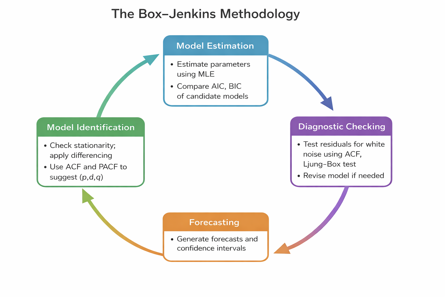
5.3.1 Box-Jenkins methodology
The Box–Jenkins methodology is a systematic approach used to identify, estimate, and validate ARIMA models for time series forecasting. The methodology consists of four main stages, which are often repeated iteratively until a satisfactory model is obtained.
1. Identification
The first step is to determine the appropriate structure of the ARIMA model. - Check stationarity
Examine the ACF and PACF plots to identify possible values for p and q
2. Estimation
Once candidate models are identified, the next step is to estimate its parameters. Evaluate:
Statistical significance of the parameters
Overall model fit using AIC or BIC
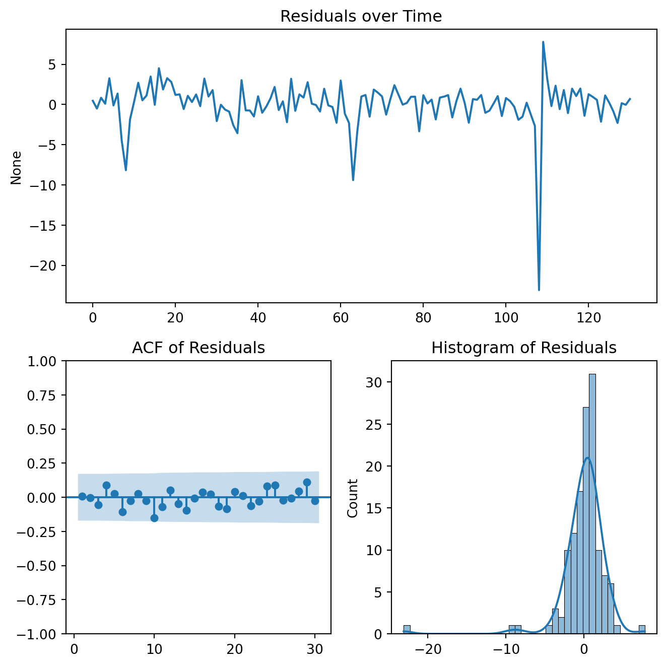
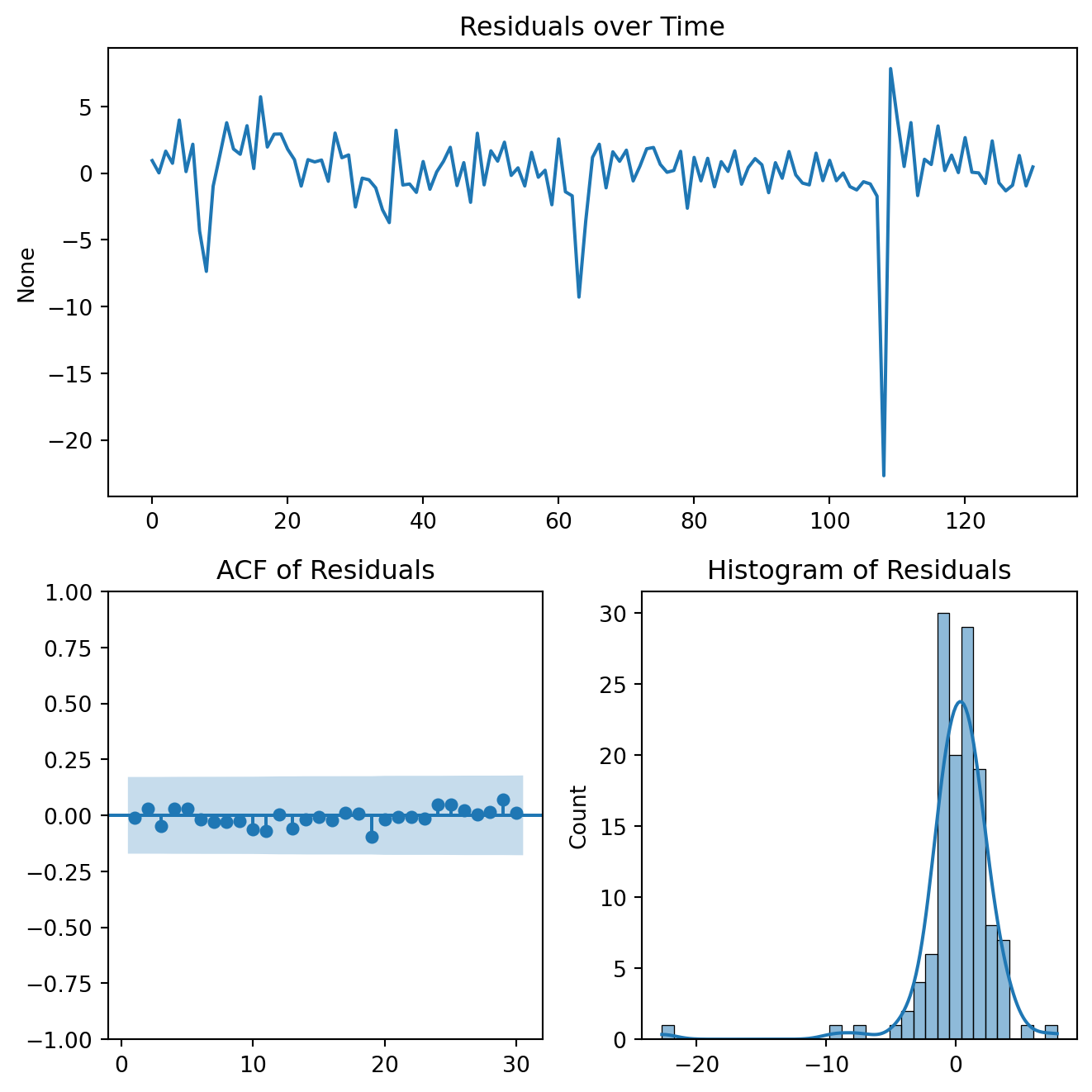
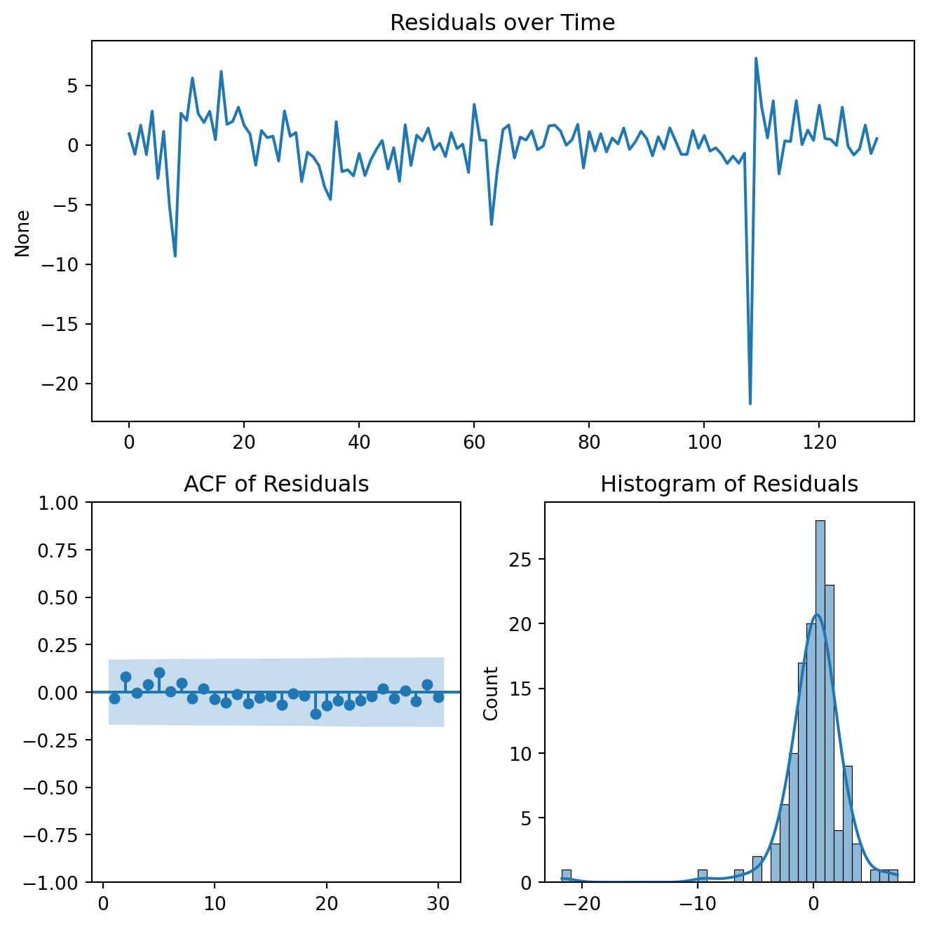
3. Diagnostic Checking
A well-specified model should produce residuals that behave like white noise. Residuals have no autocorrelation, constant variance and zero mean.
Use Residual ACF plots
Implement Ljung–Box tests for autocorrelation
Examine the residual distributions
If the residuals still contain structure or autocorrelation, the model must be re-specified, and the process returns to the identification stage.
4. Forecasting
Once a model passes the diagnostic checks, it can be used to generate forecasts.
The Box-Jenkins Methodology
NoteExample
Forecast, using ARIMA models, the GDP growth for Mexico.
Show code
import pandas as pdimport numpy as npimport matplotlib.pyplot as pltimport seaborn as snsimport statsmodels.api as smfrom datetime import datetimeimport yfinance as yffrom pandas_datareader import data as pdrfrom statsmodels.tsa.stattools import adfuller, kpssfrom statsmodels.stats.diagnostic import acorr_ljungboxfrom statsmodels.graphics.tsaplots import plot_acffrom statsmodels.graphics.tsaplots import plot_pacffrom statsmodels.tsa.arima.model import ARIMAfrom sklearn.metrics import mean_squared_errorimport plotly.graph_objects as go
/var/folders/wl/12fdw3c55777609gp0_kvdrh0000gn/T/ipykernel_69787/3857404078.py:2: InterpolationWarning:

The test statistic is outside of the range of p-values available in the
look-up table. The actual p-value is greater than the p-value returned.
Tests suggest the time series is stationary.
Plot the ACF and PACF
Show code
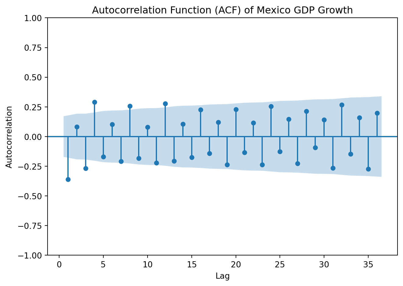
plot_acf(GDP['y'], lags=36, zero=False)plt.title('Autocorrelation Function (ACF) of Mexico GDP Growth')plt.xlabel('Lag')plt.ylabel('Autocorrelation')plt.tight_layout()plt.show()
Show code
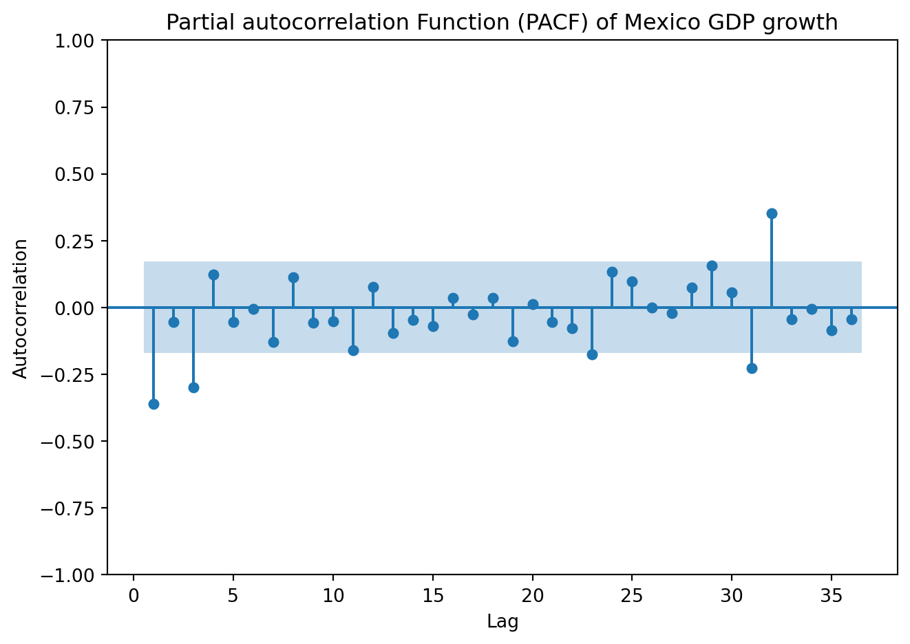
plot_pacf(GDP['y'], lags=36, zero=False, method ='ols')plt.title('Partial autocorrelation Function (PACF) of Mexico GDP growth')plt.xlabel('Lag')plt.ylabel('Autocorrelation')plt.tight_layout()plt.show()
Both the ACPF and PACF show significant spikes at lags 1 and 3, but not in lag 2. Begin by estimating an ARMA (1,1). Later, we’ll fit other models with nearby lag lengths to compare information criteria.
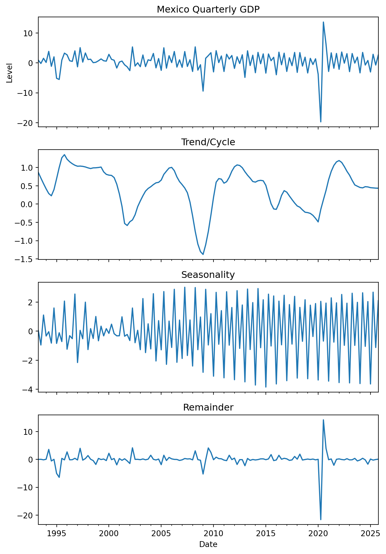
A seasonal ARIMA (sARIMA) model is formed as an ARIMA model that adds seasonal terms. These models are designed to handle repeated seasonal patterns in data, such as quarterly demand cycles, monthly sales peaks, or yearly production slowdowns. A SARIMA model extends the ARIMA framework by including seasonal autoregressive, differencing, and moving average components. It can be expressed as:
/var/folders/wl/12fdw3c55777609gp0_kvdrh0000gn/T/ipykernel_69787/3857404078.py:2: InterpolationWarning:

The test statistic is outside of the range of p-values available in the
look-up table. The actual p-value is greater than the p-value returned.
Tests suggest the time series is stationary.
Plot the ACF and PACF
Show code
plot_acf(GDP['y'], lags=36, zero=False)plt.title('Autocorrelation Function (ACF) of Mexico GDP Growth')plt.xlabel('Lag')plt.ylabel('Autocorrelation')plt.tight_layout()plt.show()
Show code
plot_pacf(GDP['y'], lags=36, zero=False, method ='ols')plt.title('Partial autocorrelation Function (PACF) of Mexico GDP growth')plt.xlabel('Lag')plt.ylabel('Autocorrelation')plt.tight_layout()plt.show()
For the nonseasonal component we found earlier that a (1,0,3) model capture the process with some accuracy. The significant spikes at lag 4, 8, 12 suggest a seasonal MA(3) component. Then, an initial candidate will be a SARIMA \((1, 0, 3) (0, 0, 3)_4\) model. Proceed to estimate the model and compare the AIC, BIC, and residuals with other reasonable guesses.
2. Estimation
def fit_sarima(ts, p, d, q, P, D, Q, s): model = SARIMAX(ts, order=(p, d, q), seasonal_order=(P, D, Q, s)) fitted_model = model.fit(disp=False)print(f"\nSARIMA({p},{d},{q})({P},{D},{Q})[{s}]")print(f"AIC: {fitted_model.aic:.2f}")print(f"BIC: {fitted_model.bic:.2f}")return fitted_model
/opt/anaconda3/lib/python3.12/site-packages/statsmodels/base/model.py:607: ConvergenceWarning:

Maximum Likelihood optimization failed to converge. Check mle_retvals
/opt/anaconda3/lib/python3.12/site-packages/statsmodels/base/model.py:607: ConvergenceWarning:

Maximum Likelihood optimization failed to converge. Check mle_retvals
Select the model with lowest information criteria.
Apply the Box–Jenkins methodology to model and forecast the series Mexican Auto Imports (MAUINSA) obtained from the FRED database from 2010 to 2026. Automotive imports/exports are closely linked to economic activity, exchange rate movements, and the structure of North American supply chains. As a result, forecasting this series can provide valuable insights into future manufacturing demand, trade dynamics, and the broader business cycle in Mexico. Reliable forecasts of auto imports may therefore be useful for firms involved in logistics and manufacturing planning, as well as for policymakers monitoring external sector activity and industrial production
5.5 SARIMAX
Up to this point, we have modeled time series using ARIMA/SARIMA models, which rely exclusively on the past behavior of the variable of interest. In many applications, however, the evolution of a time series is also driven by external factors. To incorporate this idea, we can now introduce the SARIMAX model, where the ‘X’ stands for exogenous variables.
An exogenous variable \(X_t\) affects \(Y_t\), but is not determined by the model itself. For example: policy interventions, economic indicators, or temporary shocks (e.g., pandemic dummy). As in multiple regression models, to chose \(X\) we rely on economic theory, reasoning, literature review, institutional knowledge, and data availability.
A SARIMAX \((p,d,q)(P,D,Q)_s\) model is defined as:
\[
Y_t = SARIMA + \beta X+ \varepsilon_t
\]
\(\beta X\) captures the effect of external variables, the term shifts the level of the series depending on \(X\).
In short, while SARIMA assumes the series evolves only from its own past, SARIMAX allows external variables to influence the series directly.
A SARIMAX model can also be expressed as a regression model where the residuals follow a SARIMA process:
\[
Y_t = \beta X+ u_t
\]
where:
\[
u_t \sim SARIMA(p,d,q)(P,D,Q)_s
\]
The regression component captures systematic external effects and the SARIMA component models remaining dependence and structure.
Including exogenous variables improves the model only if those variables are known or can be forecasted.
If \(X_{t+h}\) is known forecasting is straightforward
If \(X_{t+h}\) is unknown it must be assumed or forecasted
Consider as an example a simple AR1 model for GDP Growth with a temporary covid shock. That is a SARIMAX(1,0,0)(0,0,0) model with a dummy variable for periods during the covid pandemic:
with \(D=1\) for covid quarters and \(D=0\) otherwise, \(\phi_1\) captures the persistence in GDP growth \(\beta\) is the effect of the shock. \(\phi_0\) was omitted to simplify the notation.
Interpretation
With \(D=1\):
\[
Y_t = \phi_1 Y_{t-1} + \beta + \varepsilon_t
\] The series, growth, is shifted by \(\beta\).
With \(D=0\):
\[
Y_t = \phi_1 Y_{t-1} + \varepsilon_t
\]
Standard AR(1) behavior.
NoteExample
Forecast, using a SARIMAX model, the GDP growth for Mexico.
Show code
import pandas as pdimport numpy as npimport matplotlib.pyplot as pltimport seaborn as snsimport statsmodels.api as smfrom datetime import datetimeimport yfinance as yffrom pandas_datareader import data as pdrfrom statsmodels.tsa.stattools import adfuller, kpssfrom statsmodels.stats.diagnostic import acorr_ljungboxfrom statsmodels.graphics.tsaplots import plot_acf, plot_pacffrom statsmodels.tsa.arima.model import ARIMAfrom statsmodels.tsa.statespace.sarimax import SARIMAXfrom statsmodels.tsa.seasonal import seasonal_decompose, STLfrom sklearn.metrics import mean_squared_errorimport plotly.graph_objects as go
/var/folders/wl/12fdw3c55777609gp0_kvdrh0000gn/T/ipykernel_69787/1650264032.py:2: InterpolationWarning:

The test statistic is outside of the range of p-values available in the
look-up table. The actual p-value is greater than the p-value returned.
Tests suggest the time series is stationary.
Plot the ACF and PACF
Show code
plt.figure(figsize=(7, 5))plot_acf(GDP['y'], lags=36, zero=False)plt.title('Autocorrelation Function (ACF) of Mexico GDP Growth')plt.xlabel('Lag')plt.ylabel('Autocorrelation')plt.tight_layout()plt.show()
<Figure size 672x480 with 0 Axes>
Show code
plt.figure(figsize=(7, 5))plot_pacf(GDP['y'], lags=36, zero=False, method ='ols')plt.title('Partial autocorrelation Function (PACF) of Mexico GDP growth')plt.xlabel('Lag')plt.ylabel('Autocorrelation')plt.tight_layout()plt.show()
<Figure size 672x480 with 0 Axes>
2. Estimation
Define the exogenous factors. Here we will only include a dummy variable that accounts for periods of economic disruptions:
GDP['shock'] =0shock_period = [ ('2008Q2', '2009Q2'), # Global financial crisis ('2020Q1', '2021Q1') # COVID shock ]for start, end in shock_period: GDP.loc[start:end, 'shock'] =1
def fit_sarimax(ts, exog, p, d, q, P, D, Q, s): model = SARIMAX( ts, exog=exog, order=(p, d, q), seasonal_order=(P, D, Q, s), enforce_stationarity=False, enforce_invertibility=False ) fitted_model = model.fit(disp=False)print(f"\nSARIMAX({p},{d},{q})({P},{D},{Q})[{s}]")print(f"AIC: {fitted_model.aic:.2f}")print(f"BIC: {fitted_model.bic:.2f}")return fitted_model
To maintain comparability we will only estimate the \(SARIMA(1,0,1)(1,0,1)_4\) that offered the lowest information criteria earlier in section 5.4.
X = GDP[['shock']]model = fit_sarimax(GDP['y'],X,1,0,1,1,0,1,4)
model_df is the number of parameters: p+q+P+Q+k, where k is the number of exogenous coefficients. The Ljung–Box statistic at lag h is compared to a \(\chi^2\) distribution with: \(df = h − model\_df\). To be positive, we must set lags > model_df.
The null hypothesis of no serial correlation can’t be rejected.
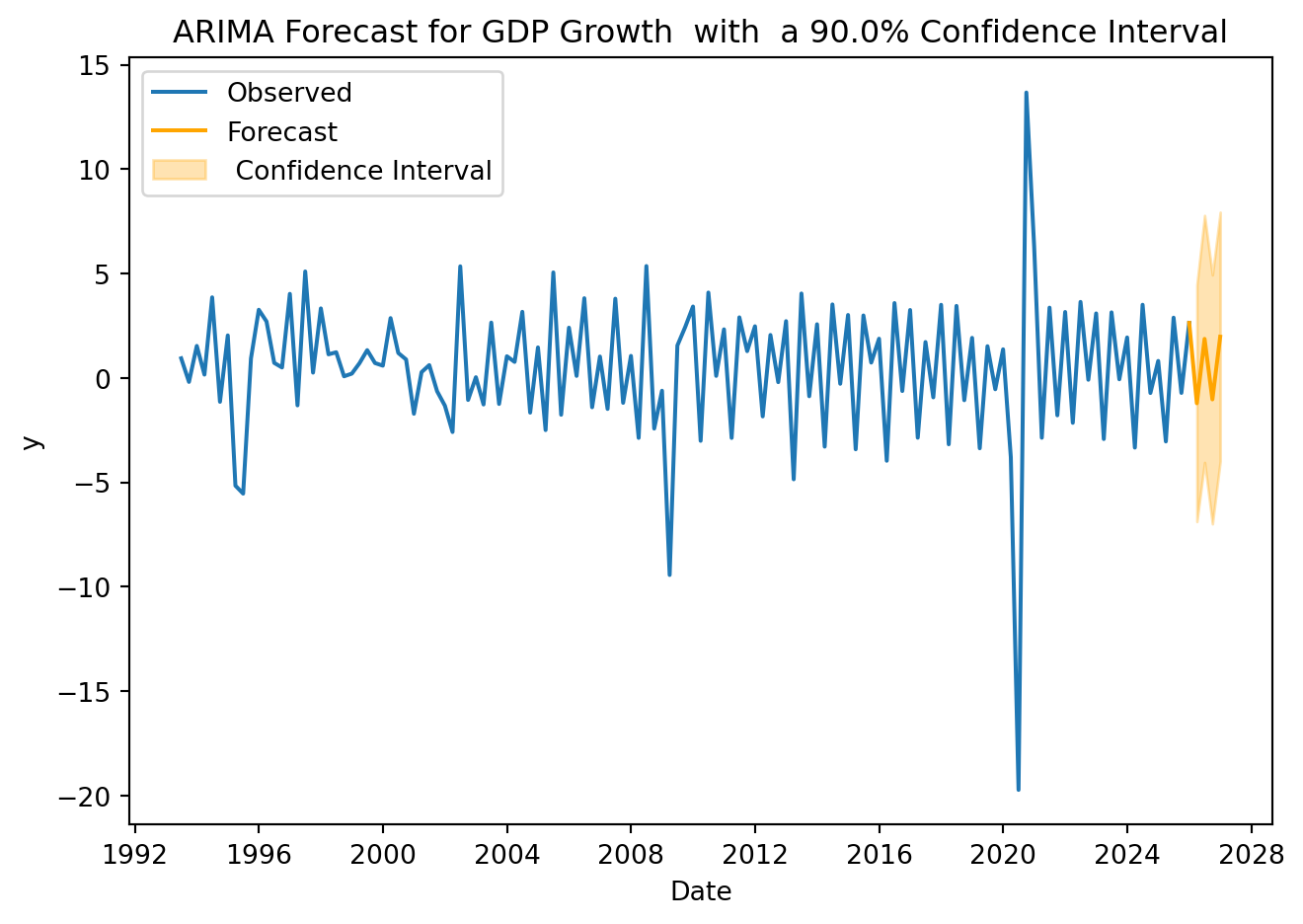
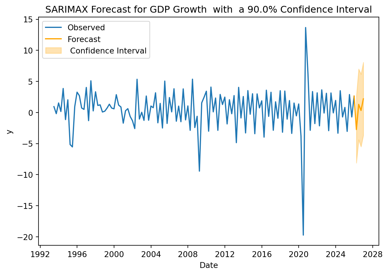
4. Forecasting
Assume that no crisis are expected for the period to be forecasted, that is, \(D_{T+h}= 0\)
periods =4cl =0.9# confidence levelfuture_X = pd.DataFrame({'shock': [0] * periods})forecast = model.get_forecast(steps=periods, exog=future_X, alpha=1-cl)mean_forecast = forecast.predicted_meanconf_int = forecast.conf_int()for date, value in mean_forecast.items():print(f"{date}: {value:.2f}")
Using monthly data from 2010 to 2025, estimate a SARIMAX model to forecast the growth rate of Mexican auto imports (MAUINSA). The dependent variable must be specified as the growth rate, computed as the first difference of the logarithm multiplied by 100. As an exogenous variable, include the growth rate of the US Industrial Production Index (INDPRO), constructed using the same transformation. Use the SARIMA specification previously identified for this series and extend it to a SARIMAX model by incorporating the exogenous regressor. Then, generate forecasts for the next 12 periods. Since SARIMAX requires future values of the exogenous variable, you must explicitly define the path of the Industrial Production Index during the forecast horizon (e.g., assume it remains constant at its most recent value or follows its recent average growth).