import pandas            as pd
import numpy             as np
import matplotlib.pyplot as plt
import seaborn           as sns
import statsmodels.api as sm1 Simple Regression Model
We are interested in studying how a variable \(y\) varies when another variable \(x\) changes. A simple equation that captures this relationship can be written as:
\[ y= \beta_0+\beta_1x +u \] where:
\(y\) is the dependent variable. It is also called the explained, response, or predicted variable.
\(x\) is the independent variable. It is also called the explanatory, control, or predictor variable.
The term \(u\) represents factors other than \(x\) that also affect \(y\). It’s often called the error term or the disturbance in the relationship.
\(\beta_1\) measures how \(y\) responds to changes in \(x\), as long as \(\frac{\Delta u}{\Delta x} =0\),
\[ \frac{\Delta y}{\Delta x}= \beta_1 \]
- \(\beta_0\) is the intercept or constant term.
By restricting how \(u\) is related to the explanatory variable \(x\), it is possible to estimate the ceteris paribus effect of \(x\) on \(y\). The zero conditional mean independence assumption:
\[ E[u|x]=E[u]=0 \]
requires that the average level of \(u\) is the same, regardless of the value of \(x\). In turn, it implies that the population regression function (PRF) is a linear function of \(x\): \[ E[y|x] = \beta_0 + \beta_1x \] It means that a one-unit increase in \(x\) changes the expected value of \(y\) by the amount \(\beta_1\).
1.1 The OLS estimator
The aim is to estimate the values of \(\beta_0\) and \(\beta_1\).
Requires a random sample of size n from the population of interest. Let \(\{x_i,y_i\}: i = 1, 2, \dots, n\), be the selected sample.
The simple linear regression can be written as: \[ y_i = \beta_0 + \beta_1 x_i + u_i \]
Define the regression residuals: \[ u_i = y_i - \hat{y_i} \]
Minimize the sum of squared residuals with respect to \(\beta_0\) and \(\beta_1\): \[ min_{\hat{\beta}_0, \hat{\beta}_1} \sum_{i=1}^n {(y_i-\hat{\beta}_0} - \hat{\beta}_1x_i)^2 \]
The resulting Ordinary Least Squares (OLS) estimates of \(\beta_0\) and \(\beta_1\) are: \[ \hat{\beta}_1 =\frac{\sum_{i=1}^n (x_i-\bar{x})(y_i-\bar{y})}{\sum_{i=1}^n (x_i-\bar{x})^2} \]
\[ \hat{\beta}_0 = \bar{y}-\hat{\beta}_1 \bar{x} \]
With the estimates, we can form the OLS regression line: \[ \hat{y_i}= \hat{\beta_0} +\hat{\beta_1}x_i \] which is also called the Sample Regression Function (SRF).
The intercept, \(\hat{\beta}_0\), is the predicted value of \(y\) when \(x\) is 0. The slope estimate, \(\hat{\beta}_1\) is the amount by which \(y\) changes when \(x\) increases by one unit.
NoteApplication in Python
Data come from the Mexican National Survey of Financial Inclusion (2021). Although there are 13,554 total observations, for the purposes of this exercise we select only the working population with a fixed income, who possessed a credit card, leaving 1,209 valid observations. Save the data in a csv file named DataENIF.
Create the variables:
education: Education level (00, none; 01, kinder; 02, elementary; 03 junior high school; 06 high school; 07 , technical; 08, bachelor; 09, postgraduate)
marital: Marital status [1 if married]
sex: Sex[1 if male]
age: age in years
income: monthly income in pesos
householdSize: number of people in the household
useCard: use of credit card per month
dPhone: owns a smartphone [1 if yes]
villageSize: [1: >=100,000 people; 2: 15,000 - 99,999; 3: 2,500 - 14,999; 4: <2500]
region: [1: Northwest; 2: Northeast; 3: West; 4: Mexico city; 5: South-center; 6: South]
We want to explain how the age of Mexicans affects their level of income. Consider the simple model:
\[ Income_i = \beta_0 +\beta_1 Age_i + u_i \]
1.1.1 Data exploration
data = pd.read_csv("DataENIF.csv")
data = data.dropna()
data.loc[:, 'income'] /= 1000

# Get rid of outliers
mean_income = data['income'].mean()
sd_income   = data['income'].std()
Lo = mean_income - 3 * sd_income
Up = mean_income + 3 * sd_income
data = data[(data['income'] > Lo) & (data['income'] < Up)]

# Select region 1
data = data[data['villageSize'] == 1]plt.figure(figsize=(8, 5))
sns.scatterplot(x=data['age'], y=data['income'], alpha=0.5)
plt.xlabel("Age")
plt.ylabel("Income (in thousand pesos)")
plt.show()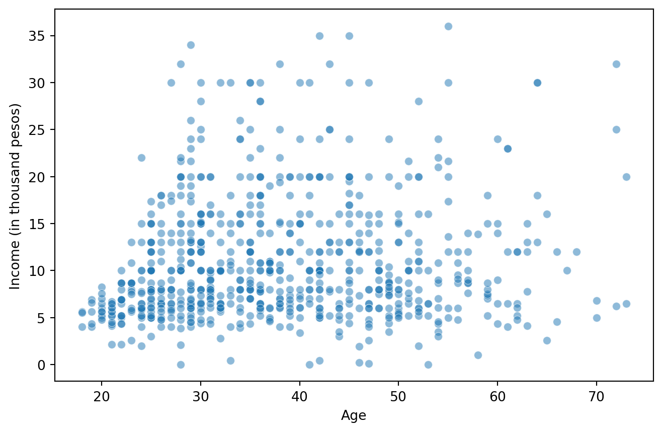
1.1.2 Estimate the model
X = data['age']     # Independent variable
Y = data['income']  # Dependent variable
X = sm.add_constant(X)  # Add an intercept term

model = sm.OLS(Y, X).fit()
print(model.summary())
OLS Regression Results
==============================================================================
Dep. Variable: income R-squared: 0.015
Model: OLS Adj. R-squared: 0.014
Method: Least Squares F-statistic: 11.48
Date: Thu, 23 Apr 2026 Prob (F-statistic): 0.000739
Time: 15:25:02 Log-Likelihood: -2456.8
No. Observations: 751 AIC: 4918.
Df Residuals: 749 BIC: 4927.
Df Model: 1
Covariance Type: nonrobust
==============================================================================
coef std err t P>|t| [0.025 0.975]
------------------------------------------------------------------------------
const 8.3807 0.787 10.651 0.000 6.836 9.925
age 0.0673 0.020 3.389 0.001 0.028 0.106
==============================================================================
Omnibus: 157.649 Durbin-Watson: 1.970
Prob(Omnibus): 0.000 Jarque-Bera (JB): 279.445
Skew: 1.267 Prob(JB): 2.09e-61
Kurtosis: 4.585 Cond. No. 134.
==============================================================================
Notes:
[1] Standard Errors assume that the covariance matrix of the errors is correctly specified.Intercept: 8.381
Slope: 0.067Interpretation: A one-year increase in age is associated with a, ceteris paribus, change of
$67.35in income.
data['predicted_income'] = model.predict(X)
sns.lineplot(x=data['age'], y=data['predicted_income'], color='red', label="Fitted Line")
sns.scatterplot(x=data['age'], y=data['income'], alpha=0.5)
plt.xlabel("Age")
plt.ylabel("Income (in thousand pesos)")
plt.title("Fitted Regression Line")
plt.legend()
plt.show()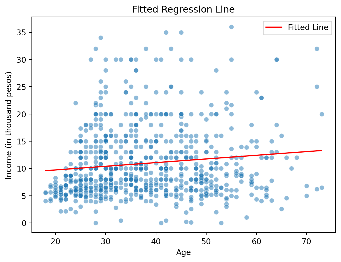
1.1.3 Prediction
new_ages = pd.DataFrame({'age': [25, 40, 70]})
new_ages = sm.add_constant(new_ages)
predictions = model.predict(new_ages)
Predicted income for age 25: $10,064.43
Predicted income for age 40: $11,074.65
Predicted income for age 70: $13,095.091.2 Goodness-of-fit
We’d like to measure how well the independent variable, \(x\), explains the dependent variable, \(y\). Define the following measures of variation:
Total sum of squares [SST]:
\[ \sum_{i=1}^n({y}_i - \bar{y})^2 \]
Explained sum of squares [SSE]:
\[ \sum_{i=1}^n(\hat{y}_i - \bar{y})^2 \]
Residual sum of squares [SSR]:
\[ \sum_{i=1}^n(y_i - \hat{y})^2 = \sum_{i=1}^n \hat{u}_i \]
Then, \[ SST= SSE + SSR \]
The fraction of total variation in \(y\) that is explained by the regression is the \(R^2\): \[ R^2 = \frac{SSE}{SST}= 1-\frac{SSR}{SST} \]
By construction, the \(R^2\) values range from 0 to 1. A higher value (closer to 1) indicates that the model explains a large proportion of the variability in the dependent variable, while a lower value (closer to 0) suggests that the independent variable does not explain much of the variation in the dependent variable.
In the example:
# Display model summary
print(model.summary())
OLS Regression Results
==============================================================================
Dep. Variable: income R-squared: 0.015
Model: OLS Adj. R-squared: 0.014
Method: Least Squares F-statistic: 11.48
Date: Thu, 23 Apr 2026 Prob (F-statistic): 0.000739
Time: 15:25:02 Log-Likelihood: -2456.8
No. Observations: 751 AIC: 4918.
Df Residuals: 749 BIC: 4927.
Df Model: 1
Covariance Type: nonrobust
==============================================================================
coef std err t P>|t| [0.025 0.975]
------------------------------------------------------------------------------
const 8.3807 0.787 10.651 0.000 6.836 9.925
age 0.0673 0.020 3.389 0.001 0.028 0.106
==============================================================================
Omnibus: 157.649 Durbin-Watson: 1.970
Prob(Omnibus): 0.000 Jarque-Bera (JB): 279.445
Skew: 1.267 Prob(JB): 2.09e-61
Kurtosis: 4.585 Cond. No. 134.
==============================================================================
Notes:
[1] Standard Errors assume that the covariance matrix of the errors is correctly specified.We can extract the \(R^2\) as follows:
r_squared = model.rsquared
print(f"R-squared: {100*r_squared:.1f}")
R-squared: 1.5Interpretation The \(R^2\) indicates that only
1.5%of the variation in income is explained by age, suggesting that other variables (such as education, experience, or location) might be more relevant predictors.
1.3 Nonlinearities
Linear regression assumes a constant relationship between the independent variable and the dependent variable. However, in many real-world cases, the relationship between variables is not strictly linear. Some popular nonlinear transformations are:
The log-level (semi-logarithmic) model:
\[ log(y) = \beta_0+\beta_1x +u \]
the interpretation of \(\beta_1\) changes as now: \[ \beta_1 = \frac{\Delta log(y)}{\Delta x} = \frac{\frac{\Delta y}{y}}{\Delta x} = \frac{\Delta \% y}{\Delta x} \]
The level-log model: \[ y = \beta_0+\beta_1 log(x) +u \]
the interpretation of \(\beta_1\) changes as now: \[ \beta_1 = \frac{\Delta y}{\Delta x / x} = \frac{\Delta y}{\Delta \% x} \]
The log-log (constant elasticity) model: \[ log(y) = \beta_0+\beta_1 log(x) +u \]
the interpretation of \(\beta_1\) changes as now: \[ \beta_1 = \frac{\Delta y / y }{\Delta x / x} = \frac{\Delta \% y}{\Delta \% x} \]
If instead of the original (lin-lin) model, we are interested in its log-level form, we need to estimate:
\[ log(Income_i) =\beta_0 + \beta_1 Age_i + u_i \] In python:
data['log_income'] = np.log(data['income'])
X = sm.add_constant(data['age'])
Y = data['log_income']
semi_log_model = sm.OLS(Y, X).fit()
print(semi_log_model.summary())
OLS Regression Results
==============================================================================
Dep. Variable: log_income R-squared: 0.005
Model: OLS Adj. R-squared: 0.004
Method: Least Squares F-statistic: 3.797
Date: Thu, 23 Apr 2026 Prob (F-statistic): 0.0517
Time: 15:25:02 Log-Likelihood: -815.84
No. Observations: 751 AIC: 1636.
Df Residuals: 749 BIC: 1645.
Df Model: 1
Covariance Type: nonrobust
==============================================================================
coef std err t P>|t| [0.025 0.975]
------------------------------------------------------------------------------
const 2.0422 0.088 23.077 0.000 1.868 2.216
age 0.0044 0.002 1.949 0.052 -3.27e-05 0.009
==============================================================================
Omnibus: 571.303 Durbin-Watson: 2.019
Prob(Omnibus): 0.000 Jarque-Bera (JB): 17620.228
Skew: -3.087 Prob(JB): 0.00
Kurtosis: 25.912 Cond. No. 134.
==============================================================================
Notes:
[1] Standard Errors assume that the covariance matrix of the errors is correctly specified.Interpretation: The coefficient on age represents the percentage change in income associated with a one-year increase in age. Specifically, a one-year increase in age is associated with a
0.44%change in income, holding other factors constant.
1.4 The dummy variable
A dummy variable is a numerical variable used in regression models to represent categorical data. It takes values of 0 or 1, indicating the presence or absence of a particular charateristic. Dummy variables allow us to incorporate qualitative information (e.g., gender, region, education level) into a quantitative model. The two values are used to put each unit in the population into one of two groups represented by \(x=1\) and \(x=0\).
If \(x=1\): \[ E[y|x=1] = \beta_0 + \beta_1 \]
If \(x=0\): \[ E[y|x=0] = \beta_0 \] Then: \[ E[y|x=1] - E[y|x=0] = \beta_1 \] \(\beta_1\) is the difference in the average value of \(y\) over the subpopulations with \(x=1\) and \(x=0\).
With \(Sex\) as the independent variable of interest, the model is:
\[ Income_i = \beta_0 + \beta_1 Sex_i + u_i \]
Since, \[ Sex=\left\lbrace\begin{array}{c} 1 \rightarrow ~if~Male \ \ \ \\ 0 \rightarrow if~Female \end{array}\right. \] this model will allows us to estimate the difference in average income between males and females.
X = sm.add_constant(data['sex'])
Y = data['income']
dummy_model = sm.OLS(Y, X).fit()
print(dummy_model.summary())
OLS Regression Results
==============================================================================
Dep. Variable: income R-squared: 0.008
Model: OLS Adj. R-squared: 0.006
Method: Least Squares F-statistic: 5.868
Date: Thu, 23 Apr 2026 Prob (F-statistic): 0.0157
Time: 15:25:02 Log-Likelihood: -2459.6
No. Observations: 751 AIC: 4923.
Df Residuals: 749 BIC: 4932.
Df Model: 1
Covariance Type: nonrobust
==============================================================================
coef std err t P>|t| [0.025 0.975]
------------------------------------------------------------------------------
const 10.3513 0.334 31.032 0.000 9.696 11.006
sex 1.1330 0.468 2.422 0.016 0.215 2.051
==============================================================================
Omnibus: 166.254 Durbin-Watson: 1.951
Prob(Omnibus): 0.000 Jarque-Bera (JB): 304.573
Skew: 1.312 Prob(JB): 7.29e-67
Kurtosis: 4.688 Cond. No. 2.64
==============================================================================
Notes:
[1] Standard Errors assume that the covariance matrix of the errors is correctly specified.Interpretation: The intercept \(\beta_0\) represents the average income for the reference category (sex = 0). The coefficient \(\beta_1\) represents the difference in average income between males and females.
The average income of females is:
$10,351.27while, the average income of males is:
$11,484.271.5 Statistical properties of the OLS estimator
Because the estimated regression coefficients are calculated from a random sample, they are random variables. Our interest now lies in understanding the properties of the distributions of \(\beta_0\) and \(\beta_1\) across different random samples from the population. The key questions are: 1. what the estimators will estimate on average?, and 2. How large their variability will be in repeated samples?.
To answer these questions, we need to establish certain assumptions. These are the standard assumptions for the linear regression model:
Assumption 1. Linear in parameters.
The relationship between \(y\) and \(x\) in the population is linear.
Assumption 2. Random sampling.
The data is a random sample drawn from the population, therefore each data point follows the population equation
Assumption 3. Sample variation in the explanatory variables
\[ \sum_{i=1}^n (x_i - \bar{x})^2>0 \]
Assumption 4. Zero conditional mean \[ E[u_i|x_i]= E[u_i]= 0 \] The value of the explanatory variable contains no information about the mean of \(u\).
Under these four assumptions:
ImportantTheorem. Unbiasedness of OLS
\[ E(\hat{\beta}_0) = \beta_0 \]
and
\[ E(\hat{\beta}_1) = \beta_1 \]
The estimated coefficients may be smaller or larger, depending on the sample that is the result of a random draw from the population. But, on average, they will be equal to the values that characterize the true relationship between \(y\) and \(x\) in the population.
Next, we’d like to know how far we can expect \(\beta_0\) and \(\beta_1\) to be away from their true population values, on average. This is called sample variability and is measured by the variance estimators, \(Var(\hat{\beta}_0)\) and \(Var(\hat{\beta}_1)\). An additional assumption is needed.
Assumption 5. Homoskedasticity. The error \(u\) has the same variance given any value of the explanatory variable, \(Var(u_i|x_i) = \sigma^2\).
The value of the explanatory variable, contains no information about the variability of the unobserved factors.
Assumptions 1-5, imply:
ImportantTheorem. Variances of the OLS estimators
\[ Var(\hat{\beta}_1) = \frac{\sigma^2}{SST_x} \]
and
\[ Var(\hat{\beta}_0) = \frac{\Sigma_{i=1}^n x_i^2}{n}\frac{\sigma^2 }{SST_x} \] where \(SST_x=\Sigma_{i=1}^n(x_i-\bar{x})^2\).
The sampling variability of the estimated regression coefficients will be the higher, the larger the variability of the unobserved factors, and the lower, the higher the variation in the explanatory variable.
Since \(\sigma^2\) is unknown, it needs to be estimated, which will then allow us to estimate \(Var(\hat{\beta}_0)\) and \(Var(\hat{\beta}_1)\). An unbiased estimate of the error variance can be obtained by calculating the variance of the residuals in the sample and subtracting the number of estimated regression coefficients from the number of observations: \[
\hat{\sigma}^2 =\ \frac{1}{n-2}\sum_{i=1}^n \hat{u}_i^2 \ =\ \frac{SSR}{n-2}
\]
ImportantTheorem. Unbiasedness of the error variance
\[ E(\hat{\sigma}^2) = \sigma^2 \]
So, the standard errors for the regression coefficients are:
\[ se(\hat{\beta}_1)= \sqrt{Var(\hat{\beta_1})} = \sqrt{\frac{\hat{\sigma}^2}{SST_x}} \] and
\[ se(\hat{\beta}_0)= \sqrt{Var(\hat{\beta_0})} = \sqrt{\frac{\hat{\sigma}^2 }{SST_x}\frac{\Sigma_{i=1}^n x_i^2}{n}} \]
In the table of OLS Regression Results, the standard errors are shown in the column std err.