import pandas            as pd
import numpy             as np
import matplotlib.pyplot as plt
import seaborn           as sns
import statsmodels.api   as sm
import scipy.stats as stats2 Multiple Linear Regression
The Assumption 4 in the simple regression model will frequently fail because it ignores other factors that simultaneously affect the dependent variable, but were left in the error term. In most real-world scenarios, outcomes are influenced by multiple factors. We can incorporate these factors in a Multiple Linear Regression (MLR) model, allowing us to better capture the complexity of economic relationships.
The general multiple regression model can be written in the population as \[ y=\beta_0+\beta_1x_1 +\beta_2x_2 + \beta_3x_3 + \dots + \beta_k x_k +u \] It describes an underlying population and depends on unknown parameters.
What is the meaning of \(\beta_j\)?
\[ \frac{\Delta y}{\Delta x_j}= \beta_j \] \(\beta_j\) indicates by how much the dependent variable \(y\) changes when the independent variable \(x_j\) changes by one unit, ceteris paribus.
In a multiple regression model, the zero conditional mean assumption is more likely to hold because fewer factors are placed in the error.
2.1 Estimation
Once we have a sample data we can estimate the parameters employing an estimation method, such as ordinary least squares. Let \(\{y_i,x_{1i}, x_{2i}, \cdots, x_{ki}\}: i = 1, 2, \dots, n\), be the selected sample.
- Define the regression residuals:
\[ u_i = [y_i - \hat{y_i}] = [y_i - \hat{\beta}_0 - \hat{\beta}_1x_{i1} -\hat{\beta}_2x_{i2}- \dots - \hat{\beta}_kx_{ik}] \]
- Minimize the sum of squared residuals:
\[ min_{\hat{\beta}_0, \hat{\beta}_1, \cdots, \hat{\beta}_k} \sum_{i=1}^n \big(y_i-\hat{\beta}_0 - \hat{\beta}_1x_{i1} -\hat{\beta}_2x_{i2}- \dots - \hat{\beta}_kx_{ik}\big)^2 \] to obtain the OLS estimators.
- The fitted values from the regression are:
\[ \hat{y} = \hat{\beta}_0 +\hat{\beta}_1 x_1 + \hat{\beta}_2 x_2+\dots +\hat{\beta}_k x_k \]
NoteApplication in Python
We will continue employing the case of Financiera Ma, to estimate a multiple linear regression model that explains the income level of mexicans. The model of interest is:
\[ Income_i = \beta_0 +\beta_1 Age_i + \beta_2 Sex_i + \beta_3 HouseholdSize_i + u_i \]
Import the libraries
Load and clean the data
data = pd.read_csv("DataENIF.csv")
data = data.dropna()
data.loc[:, 'income'] /= 1000

mean_income = data['income'].mean()
sd_income   = data['income'].std()
Lo = mean_income - 3 * sd_income
Up = mean_income + 3 * sd_income
data = data[(data['income'] > Lo) & (data['income'] < Up)]
data = data[data['villageSize'] == 1]
Estimate the MLR model
X = data[['age', 'sex','householdSize']]     # Independent variable
Y = data['income']  # Dependent variable
X = sm.add_constant(X)  # Add an intercept term

mrm = sm.OLS(Y, X).fit()

print(mrm.summary())
OLS Regression Results
==============================================================================
Dep. Variable: income R-squared: 0.043
Model: OLS Adj. R-squared: 0.039
Method: Least Squares F-statistic: 11.10
Date: Thu, 23 Apr 2026 Prob (F-statistic): 3.93e-07
Time: 15:25:07 Log-Likelihood: -2446.2
No. Observations: 751 AIC: 4900.
Df Residuals: 747 BIC: 4919.
Df Model: 3
Covariance Type: nonrobust
=================================================================================
coef std err t P>|t| [0.025 0.975]
---------------------------------------------------------------------------------
const 10.1340 0.983 10.306 0.000 8.204 12.064
age 0.0559 0.020 2.826 0.005 0.017 0.095
sex 1.0710 0.460 2.327 0.020 0.167 1.975
householdSize -0.5633 0.141 -3.992 0.000 -0.840 -0.286
==============================================================================
Omnibus: 155.794 Durbin-Watson: 1.943
Prob(Omnibus): 0.000 Jarque-Bera (JB): 277.910
Skew: 1.245 Prob(JB): 4.49e-61
Kurtosis: 4.636 Cond. No. 172.
==============================================================================
Notes:
[1] Standard Errors assume that the covariance matrix of the errors is correctly specified.Interpretation:
\(\rightarrow\ \beta_1\): A one-year increase in age is associated with a, ceteris paribus, change of
$55.9in income.
\(\rightarrow\ \beta_2\): The average income difference between individuals in category 1 (Males) and 0 (Females) is
$1,071.0\(\rightarrow\ \beta_3\): ??
2.1.1 Prediction
We can use the fitted model to predict the income of a hypotethical individual. Consider the following characteristics:
# Indicate the characteristics
new_data = pd.DataFrame({'const': [1], 'age': [40], 'sex': [1], 'householdSize': [2]})

# Predict income using the estimated model
predicted_income = mrm.predict(new_data)
Predicted income: $12,315.482.1.2 Goodness-of-fit
Once we estimate a regression model, we need a way to assess how well it explains the variability in the dependent variable. The coefficient of determination, \(R^2\), measures the extent to which variation in the dependent variable is predictable from the independent variable(s).
\[ R^2 := \frac{SSE}{SST}= 1- \frac{SSR}{SST} \]
The \(R^2\) in our model is:
r2 = mrm.rsquared

print(f" R-squared: {r2:.1%}")
R-squared: 4.3%Remarks:
\(\rightarrow\) As the \(SSR\) never increases when additional regressors are added to the model, the \(R^2\) never decreases (unless the coefficient on the added regressor is zero).
\(\rightarrow\) Higher \(R^2\) values indicate a better fit, but it does not imply causality.
\(\rightarrow\) A low \(R^2\) does not preclude precise estimation of partial effects.
To increase the \(R^2\) one may be tempted to simply add more predictors to the regression model (even if they are irrelevant), this is called overfitting. To address this issue, we introduce the \(Adjusted \ R^2\) as a new measure of goodness-of-fit, which accounts for the number of predictors (\(k\)) and penalizes unnecessary complexity.
\[ \text{adjusted } R^2 = 1-(1-R^2)\frac{n-1}{n-k-1} \] increases only if the higher \(R^2\) is more than what it would be expected by chance.
The \(Adjusted \ R^2\) in our model is:
adj_r2 = mrm.rsquared_adj

print(f"Adjusted R-squared: {adj_r2:.1%}")
Adjusted R-squared: 3.9%2.1.3 Polynomials
So far, we have assumed that the relationship between the dependent variable \(Y\) and the independent variables \(X\) is linear. However, in many real-world cases, relationships between variables are nonlinear. This was clear in Figure 1.1 when we try to capture the relationship between age and income with a straight-line. To allow for curvature in the relationship, we can extend our regression model by including polynomial terms of the independent variables.
The polynomial regression model of degree \(k\) takes the form:
\[ y = \beta_0 + \beta_1x+\beta_2x^2+\beta_3x^3+\dots+\beta_kx^k+u \]
However, overfitting can occur if the polynomial degree is too high. A curved relationship between \(X\) and \(Y\) is allowed with a simpler second-degree (quadratic) polynomial regression model:
\[ y = \beta_0 + \beta_1x+\beta_2x^2+u \]
The partial effects of \(X\) on \(Y\) is given by the derivative of the equation:
\[ \frac{\partial y}{\partial x} = \beta_1+2\beta_2x \] This means that the effect of \(X\) on \(Y\) depends on \(X\) itself.
\(\rightarrow\) When \(\beta_1>0\) and \(\beta_2<0\), the curve has a parabolic shape (concave).
\(\rightarrow\) When \(\beta_1<0\) and \(\beta_2>0\), the curve is U-shaped (convex).
NoteApplication in Python
A multiple linear regression model with polynomials is used to explain the income level of mexicans. The model of interest is:
\[ Income_i = \beta_0 +\beta_1 Age_i +\beta_2 Age^2_i + \beta_3 Sex_i + \beta_4 HouseholdSize_i + u_i \]
# Create the polynomial term (age squared)
data['age2'] = data['age'] ** 2

X = data[['age', 'age2', 'sex', 'householdSize']]
Y = data['income']

X = sm.add_constant(X)

mrm2 = sm.OLS(Y, X).fit()

print(mrm2.summary())
OLS Regression Results
==============================================================================
Dep. Variable: income R-squared: 0.061
Model: OLS Adj. R-squared: 0.056
Method: Least Squares F-statistic: 12.13
Date: Thu, 23 Apr 2026 Prob (F-statistic): 1.48e-09
Time: 15:25:07 Log-Likelihood: -2438.9
No. Observations: 751 AIC: 4888.
Df Residuals: 746 BIC: 4911.
Df Model: 4
Covariance Type: nonrobust
=================================================================================
coef std err t P>|t| [0.025 0.975]
---------------------------------------------------------------------------------
const 1.6543 2.423 0.683 0.495 -3.102 6.411
age 0.5114 0.121 4.235 0.000 0.274 0.748
age2 -0.0055 0.001 -3.822 0.000 -0.008 -0.003
sex 1.1423 0.456 2.502 0.013 0.246 2.038
householdSize -0.5949 0.140 -4.246 0.000 -0.870 -0.320
==============================================================================
Omnibus: 159.077 Durbin-Watson: 1.958
Prob(Omnibus): 0.000 Jarque-Bera (JB): 291.559
Skew: 1.252 Prob(JB): 4.88e-64
Kurtosis: 4.747 Cond. No. 1.97e+04
==============================================================================
Notes:
[1] Standard Errors assume that the covariance matrix of the errors is correctly specified.
[2] The condition number is large, 1.97e+04. This might indicate that there are
strong multicollinearity or other numerical problems.Note that \(\beta_1>0\) and \(\beta_2<0\), what does it mean?
betas = mrm2.params

# hypothetical values for other explanatory variables
sim_sex    = 1
sim_hhsize = data['householdSize'].mean()

# Generate a range of age values for the plot
age_values = np.linspace(data['age'].min(), data['age'].max(), 100)

# Compute predicted income with other variables set to their mean
income_values = (
    betas['const']
    + betas['age'] * age_values
    + betas['age2'] * age_values**2
    + betas['sex'] * sim_sex
    + betas['householdSize'] * sim_hhsize
)

# Create the plot
plt.figure(figsize=(7, 5))
plt.plot(age_values, income_values, color='steelblue', label="Estimated Relationship")
plt.axvline(-betas.iloc[1] / (2 * betas.iloc[2]), color='red', linestyle="--", label="Turning Point")
plt.xlabel("Age")
plt.ylabel("Predicted Income")
plt.title("Predicted Relationship Between Age and Income")
plt.legend()
plt.show()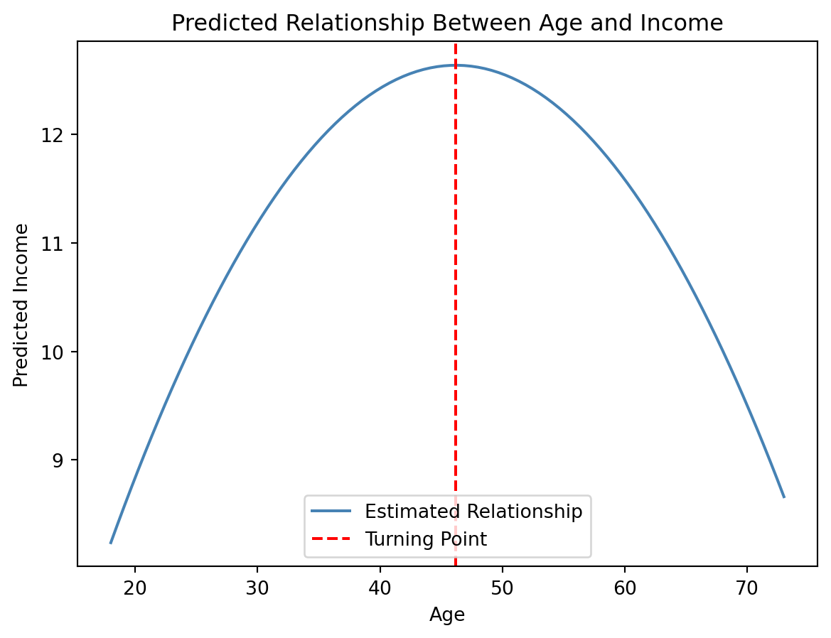
The curve is concave (inverted U-shape), meaning income increases with age at first, then declines. The turning point (max) is calculated as:
\[
x^{max}=-\frac{\hat{\beta_1}}{2\hat{\beta}_2}
\]
ageMax = -(betas['age'] / (2 * betas['age2']))

print(f"Turning point (ageMax) accurs at {ageMax:.0f}.")
Turning point (ageMax) accurs at 46.2.1.4 Statistical properties
After estimating a multiple regression model, it is essential to understand the statistical properties of the Ordinary Least Squares (OLS) estimator. These properties determine the reliability and validity of our estimates.
For OLS to be a valid estimation method, we must ensure that our data satisfies the following assumptions:
Assumption 1. Linear in parameters.
The model is linear in the parameters \(\beta_0, \beta_1, \dots, \beta_k\)
Assumption 2. Random sampling.
The data are drawn independently from the population.
Assumption 3. No perfect collinearity.
In the sample (and therefore in the population), none of the independent variables is constant and there are no exact linear relationships among the independent variables.
Typical cases when this assumption fails:
Include the same explanatory variable measured in different units
An independent variable is an exact linear function of two o more independent variables
The sample size is small relative to the number of parameters being estimated
Assumption 4. Zero conditional mean.
The error \(u\) has an expected value of zero given any values of the independent variables \[ E(u \mid x_1, \ x_2,\ x_3, \dots, \ x_k)=0 \]
Cases when this assumption fails:
- The functional relationship is misspecified
- Omitting an important factor that is correlated with any of the independent variables.
Under these four assumptions:
ImportantTheorem. Unbiasedness of OLS
\[ E(\hat{\beta}_j) = \beta_j, \ \ \ j=0,\ 1,\ 2, \dots,k \] The OLS estimators are unbiased estimators of the population parameters.
Assumption 5. Homoskedasticity.
The error u has the same variance given any value of the explanatory variables \[ Var(u|x_1,x_2,\dots,x_k) = \sigma^2 \].
The value of the explanatory variable, contains no information about the variability of the unobserved factors.
Assumptions 1 to 5 are collectively know as the Gauss-Markov assumptions.
Assumptions 1-5, imply:
ImportantTheorem. Variance of the OLS slope estimators
\[ Var(\hat{\beta}_j) = \frac{\sigma^2}{SST_j \ (1-R_j^2)} \]
for \(j=1,2,\dots,k\). Where \(SST_j=\Sigma_{i=1}^n(x_j-\bar{x})^2\) is the total sample variation on \(x_j\), and \(R^2_j\) is the R-squared from regressing \(x_j\) on all other independent variables (including the intercept).
We proceed to use data to estimate \(\sigma^2\), which will then allow us to estimate \(Var(\beta_j)\). Because \(\sigma^2=E(u^2)\), an unbiased estimator of \(\sigma^2\) is the sample average of the squared errors \(\big( \frac{\Sigma_{i=1}^nu_i^2}{n} \big)\), but we do not observe \(u\), and replacing it by \(\hat{u_i}\) leads to a biased estimator. An unbiased estimate of the error variance can be obtained by calculating the variance of the residuals and subtracting the number of estimated regression coefficients from the number of observations.
The number of observations minus the number of estimated parameters are also called the degrees of freedom.
\[ \hat{\sigma}^2 =\ \frac{1}{n-k-1}\sum_{i=1}^n \hat{u}_i^2 \ =\ \frac{SSR}{n-k-1} \]
Under the assumptions 1-5,
ImportantTheorem. Unbiasedness of the error variance
\[ E(\hat{\sigma}^2) = \sigma^2 \]
Calculation of standard errors for regression coefficients is:
\[ se(\hat{\beta}_j)= \sqrt{\hat{Var}(\hat{\beta_j})} = \sqrt{\frac{\hat{\sigma}^2}{SST_j\ (1-R_j^2)}} \]
Assumptions 1 to 5, also imply:
ImportantTheorem. Gauss-Markov Theorem
Under assumptions 1 to 5, \(\hat{\beta}_0,\hat{\beta}_1,\dots, \hat{\beta}_k\) are the Best Linear Unbiased Estimators (BLUEs) of \(\beta_0, \ \beta_1, \dots,\beta_k.\)
\(Best\) is defined as having the smallest variance. That is, for any estimator \(\tilde{\beta}\) that is linear an unbiased, \(Var(\hat{\beta}) \leq Var(\tilde{\beta}).\)
If any of the Gauss-Markov assumptions fail, then this theorem no longer holds.
Failure of the zero conditional mean assumption (4) causes OLS to be biased.
Failure of the homoskedasticity assumption (5), causes the OLS to no longer have the smallest variance among the linear unbiased estimators.
2.2 Inference
Up to now, under Gauss-Markov assumptions, we found:
OLS estimators are unbiased
Estimator of the error variance is unbiased
Variance is the smallest among linear unbiased estimators (useful for describing the precision of the estimators).
The OLS estimators are random variables, we know their mean and variance. For purposes of inference, we need the full sampling distribution, which will allow us to:
Tests hypothesis about population parameters.
Construct confidence intervals.
2.2.1 Distribution of \(\beta_j\)
The \(\beta_j\)’s are unknown features of the population. We can only hypothesize about their values, and then use statistical inference to test the validity of the hypothesis. But that requires the full distribution of the OLS estimators \(\hat{\beta}_0, \hat{\beta_1}, \dots, \hat{\beta_k}\). In order to derive their distribution an additional assumption is needed:
Assumption 6. Normality of the error term.
ImportantTheorem. Unbiasedness of OLS
The population error, \(u \backsim \ Normal\ (0, \ \sigma^2)\), independently of the explanatory variables, \(x_{1}, x_{2}, \dots , x_{k}.\)
Because \(u\) is independent of the \(x_j\) under Assumption 6, \(E(u\mid x_1,x_2, \dots, x_k) = E(u)=0\), and \(Var(u\mid x_1,x_2, \dots, x_k) = Var(u)= \sigma^2\). Therefore, A6, includes A4 and A5.
Assumptions 1 to 6 constitute the Classical Linear Model (CLM) assumptions.
ImportantTheorem. Variance of the OLS slope estimators
Under the CLM assumptions:
\[
\hat{\beta_j} \sim Normal \ \big(\beta_j,Var(\hat{\beta}_j)\big)
\]
2.2.2 The t-statistic
We now know that, under the CLM assumptions, the estimated OLS coefficients follow a normal distribution. The standarized version then follows a normal distribution with a mean of zero and variance of one, that is:
\[ \frac{\hat{\beta_j}-\beta_j}{sd(\hat{\beta_j})} \sim N(0,1) \]
As shown by the theorem on unbiasedness of the error variance, an unbiased estimator of \(sd(\hat{\beta_j})\) is \(se(\hat{\beta_j})\). When the standarization above uses the standard error, the normal distribution is replaced by the t-distribution.
For an estimated coefficient \(\hat{\beta_j}\), the t-statistic is given by:
\[ t_j = \frac{\hat{\beta_j}-\beta_j}{se(\hat{\beta_j})} \sim t_{n-k-1} \]
where:
- \(\hat{\beta_j}\) is the estimated coefficient for the \(j-th\) independent variable.
- \(\beta_j\) is the hypothesized value.
- \(se(\hat{\beta_j})\) is the standard error of \(\hat{\beta_j}\).
- \(n-k-1\) are the degrees of freedom. The difference between the sample size and the estimated parameters.
Hypothesis Testing with the t-statistic
We use the t-statistic to test hypotheses about the value of \(\beta_j\). A hypothesis of frequent interest is \(\beta_j=0\), if the hypothesis is true, \(x_j\) has no effect on the expected value of \(y\). More formally, we can use the t-statistic to test the null hypothesis:
\[ H_0: \beta_j =0 \] vs
\[ H_1: \beta_j \ne 0 \]
We’d like to find evidence to reject the null hypothesis. The larger the t-statistic, the stronger the evidence that \(\hat{\beta_j}\) is different from \(0\).
Note:
The farther the estimated coefficient is from zero, the less likely is that the null hypothesis holds true.
The size of the t-statistic depends on the variability of the estimates coefficient. The larger the variance, the lower the t-stat.
The t-stat measures how many estimated standard deviations the estimated coefficient is away from zero.
Decision Rule:
Compare the absolute value of \(t_j\) to the critical value from the t-distribution at a chosen significance level (\(\alpha\)).
\[ \text{If} \ |t_j| \ge t_{\alpha/2,df} \Rightarrow \text{Reject} \ H_0. \]
\[ \text{If} \ |t_j| < t_{\alpha/2,df} \Rightarrow \text{Fail to reject} \ H_0. \]
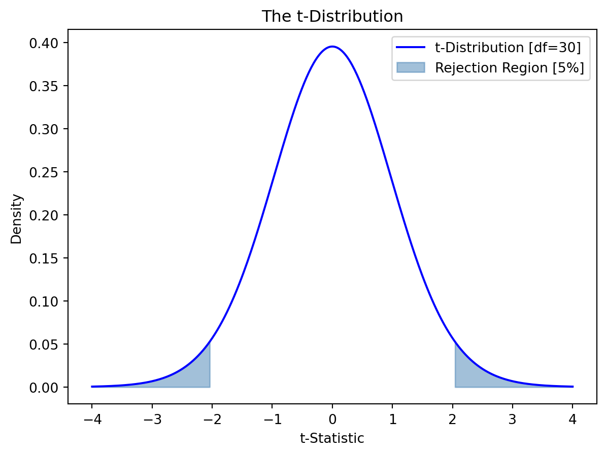
We can compute the critical values for a two-tailed test from the t distribution in python as follows:
df    = 30    # Specify the degrees of freedom
alpha = 0.05  # Specify the significance level

t_critical = stats.t.ppf(1 - alpha/2, df)

print(f"The critical t-statistic: {t_critical:.4f}")
The critical t-statistic: 2.0423Figure 2.1 below shows a t-distribution (30 degrees of freedom) with shaded rejection regions at both tails, indicating where we would reject the null hypothesis in a two-tailed test at a 5% significance level.
NoteExample
Use the estimates of the multiple linear regression model:
\[ Income_i = \beta_0 +\beta_1 Age_i +\beta_2 Age^2_i + \beta_3 Sex_i + \beta_4 HouseholdSize_i + u_i \] to test the hypothesis that the effect of \(Sex\) on \(Income\) is statistically null.
We estimated this model earlier, called it \(mrm2\)
print(mrm2.summary()) OLS Regression Results
==============================================================================
Dep. Variable: income R-squared: 0.061
Model: OLS Adj. R-squared: 0.056
Method: Least Squares F-statistic: 12.13
Date: Thu, 23 Apr 2026 Prob (F-statistic): 1.48e-09
Time: 15:25:07 Log-Likelihood: -2438.9
No. Observations: 751 AIC: 4888.
Df Residuals: 746 BIC: 4911.
Df Model: 4
Covariance Type: nonrobust
=================================================================================
coef std err t P>|t| [0.025 0.975]
---------------------------------------------------------------------------------
const 1.6543 2.423 0.683 0.495 -3.102 6.411
age 0.5114 0.121 4.235 0.000 0.274 0.748
age2 -0.0055 0.001 -3.822 0.000 -0.008 -0.003
sex 1.1423 0.456 2.502 0.013 0.246 2.038
householdSize -0.5949 0.140 -4.246 0.000 -0.870 -0.320
==============================================================================
Omnibus: 159.077 Durbin-Watson: 1.958
Prob(Omnibus): 0.000 Jarque-Bera (JB): 291.559
Skew: 1.252 Prob(JB): 4.88e-64
Kurtosis: 4.747 Cond. No. 1.97e+04
==============================================================================
Notes:
[1] Standard Errors assume that the covariance matrix of the errors is correctly specified.
[2] The condition number is large, 1.97e+04. This might indicate that there are
strong multicollinearity or other numerical problems.the coefficient estimates were stored in \(betas = mrm2.params\). Under the null,
\[ t = \frac{1.1423-0}{0.456} \]
se = mrm2.bse
t1 = (betas['sex'] - 0)/se['sex']

print(f"The calculated t-statistic is: {t1:.4f}")
The calculated t-statistic is: 2.5024Obtain the critical value as:
df    = 746    # Specify the degrees of freedom [n-k-1]
alpha = 0.05   # Specify the significance level

t_critical = stats.t.ppf(1 - alpha/2, df)

print(f"The critical value is: {t_critical:.4f}")
The critical value is: 1.9631Then at a 95% confidence level [5% significance] level, the null hypotesis is rejected, the effect of \(Sex\) on \(Income\) is statistically different from zero.
P-value
Rather than testing the hypothesis at different significant levels, we could answer the question: what is the smallest significant level at which the null hypothesis would be rejected?.
If the significance level is made smaller and smaller, there will be a point where the null hypothesis cannot be rejected anymore. The reason is that, by lowering the significance level, one wants to avoid more and more to make the error of rejecting a correct \(H_0\). The smallest significance level at which the null hypothesis is still rejected, is called the p-value of the hypothesis test. The p-value then is the significance level at which one is indifferent between rejecting and not rejecting the null hypothesis.
A small p-value is evidence against the null hypothesis because one would reject the null hypothesis even at small significance levels. A large p-value is evidence in favor of the null hypothesis.
\[ \text{If} \ p-value < \alpha \Rightarrow \text{Reject} \ H_0. \]
Calcule the p-value in python as:
# Compute one-tailed probability
prob = 1 - stats.t.cdf(abs(t1), df)

# Compute two-tailed p-value
pval = prob * 2

# Print the result
print(f"P-value: {pval:.3f}")
P-value: 0.013Guidelines for discussing economic and statistical significance
- If a variable is statistically significant, discuss the magnitude of the coefficient to get an idea of its economic or practical importance.
- The fact that a coefficient is statistically significant does not necessarily mean it is economically or practically significant!
- If a variable is statistically and economically important but has the “wrong” sign, the regression model might be misspecified.
- Conventional levels of statistical significance are 10%, 5%, or 1%
- If the sample size is small, effects might be imprecisely estimated so that the case for dropping insignificant variables is less strong.
Confidence Interval
While point estimates \(\hat{\beta_j}\) provide a single best guess, confidence intervals give a range within which the true population parameter is likely to lie.
\[ \hat{\beta}_j \pm t_{\alpha/2,df} \cdot se(\hat{\beta}_j) \] That is:
\[ P\Big( \hat{\beta}_j-t_{\alpha/2,df} \cdot se(\hat{\beta}_j) \leq \beta_j \leq \hat{\beta}_j+t_{\alpha/2,df} \cdot se(\hat{\beta}_j) \Big) = (1-\alpha)\% \] If the confidence interval excludes 0, the coefficient is statistically significant at the chosen level. If the confidence interval includes 0, we cannot rule out the possibility that the true effect is zero.
# Compute the confidence interval
b_lo = betas['sex'] - t_critical * se['sex']  # Lower bound
b_up = betas['sex'] + t_critical * se['sex']  # Upper bound

# Print the results
print(f"95% Confidence Interval for 'Sex': ({b_lo:.3f}, {b_up:.3f})")
95% Confidence Interval for 'Sex': (0.246, 2.038)2.2.3 The F-Statistic
In multiple regression analysis, with \(k\) independent variables, we might want to test whether a subgroup of the independent variables, \(q\le k\), has a statistically significant effect on the dependent variable. A test of multiple restrictions is called a multiple hypothesis test or a joint hypothesis test. Unlike the t-test, which examines individual coefficients, the F-test evaluates the jointly significance of a group of coefficients. For instance, we could be interested in testing:
\[ H_0: \beta_1=\beta_2=\cdots = \beta_q=0 \]
The F-statistic is calculated as:
\[ F=\frac{(SSR_R-SSR_{UR})/q}{SSR_{UR}/(n-k-1)} \]
where:
– \(SSR_R\) is the Sum of Squared Residuals of the “restricted” model (assuming the null is true).
– \(SSR_{UR}\) is the Sum of Squared Residuals of the “unrestricted” model (the models with all \(k\) independent vars).
– \(q\) is the number of restrictions.
Decision Rule: To determine whether to reject the null hypothesis, we ought to compare the calculated \(F-statistic\) with the critical value from the F-distribution at a chosen significance level \(\alpha\).
\[ \text{If} \ F \ge F_{\alpha,q,df} \Rightarrow \text{Reject} \ H_0. \] Alternatively,
\[ \text{If} \ p-value < \alpha \Rightarrow \text{Reject} \ H_0. \]
If the null is rejected, the subgroup of \(q\) variables explains a significant proportion of the variation in the dependent variable.
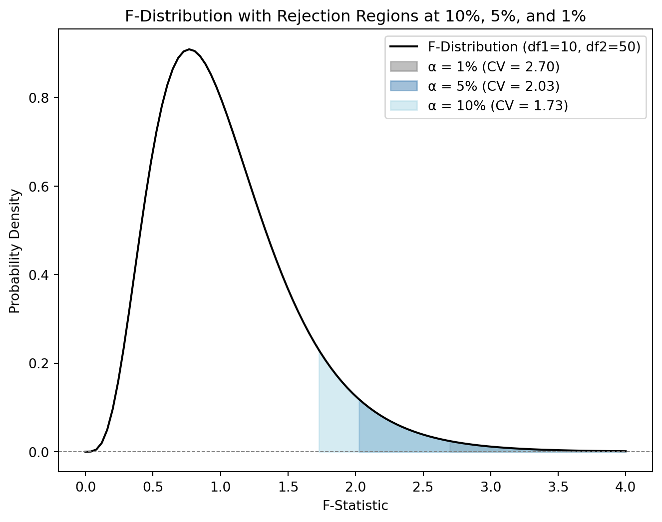
Figure 2.2 illustrates the F-distribution with 10 numerator degrees of freedom and 50 denominator degrees of freedom. The distribution is right-skewed, as is typical of F-distributions, and represents the probability density of different F-statistic values. The colored shaded areas represent the rejection regions for different significance levels (10%, 5%, and 1%). The critical value shifts to the right as the chosen significance level decreases (the confidence level increases), these are the F-statistic thresholds above which we would reject the null hypothesis.
Testing the overall fit of the model
The F-test is used to test the null hypothesis that all regression coefficients, except the intercept, are equal to zero, that is, to test the overall fit of the model. The ‘restricted’ model is simply the regression on the intercept: \[ y=\beta_0 +u \]
The null hypothesis can be written as:
\[ H_0: \beta_1=\beta_2=\dots=\beta_k=0 \] while the alternative hypothesis is that at least one of the coefficients is different from zero.
The F-statistic in this case is closely related to the coefficient of determination \((R^2)\):
\[ F=\frac{(SSR_R-SSR_{UR})/q}{SSR_{UR}/(n-k-1)} =\frac{R^2/k}{(1-R^2)/(n-k-1)} \]
This shows that the F-statistic increases as \(R^2\) increases, meaning a better-fitting model will have a larger F-statistic.
NoteExample
Use the estimates of the multiple linear regression model:
\[ Income_i = \beta_0 +\beta_1 Age_i +\beta_2 Age^2_i + \beta_3 Sex_i + \beta_4 HouseholdSize_i + u_i \] to test the hypothesis \(\beta_1=\beta_2=\beta_3=\beta_4=0\).
Step 1. Begin by obtaining the SSR of restricted model:
Y = data['income']
X = np.ones(len(Y))
model_restricted = sm.OLS(Y, X).fit()           # Estimate the model
hat_Y_restricted = model_restricted.predict(X)  # Predicted values restricted

# Calculate residuals
resid_r = Y - hat_Y_restricted

# Calculate SSR
SSR_restricted = np.sum(resid_r ** 2)
Step 2. Get the SSR of the unrestricted model:
X = data[['age', 'age2', 'sex', 'householdSize']]
Y = data['income']
X = sm.add_constant(X)
mrm2 = sm.OLS(Y, X).fit()

hat_Y_unrestricted = mrm2.predict(X)  # Predicted values unresstricted
resids_un = Y - hat_Y_unrestricted
SSR_unrestricted = np.sum(resids_un ** 2)
Step 3. Calculate the F-stat:
k  = X.shape[1]-1  # number of explanatory variables
n  = X.shape[0]    # number of observations
q  = k             # number of restrictions
F = ((SSR_restricted - SSR_unrestricted )/q)/(SSR_unrestricted/(n-k-1))

print(f"F-stat is: {F:.4f}")
F-stat is: 12.1269Step 4. Obtain the critical value
alpha = 0.05   # Significance level (for 95% confidence)
df1 = k        # Numerator degrees of freedom
df2 = n-k-1      # Denominator degrees of freedom

# Calculate the F critical value
F_critical = stats.f.ppf(1 - alpha, df1, df2)

print(f"F-critical value at 95% confidence (df1={df1}, df2={df2}): {F_critical:.4f}")
F-critical value at 95% confidence (df1=4, df2=746): 2.3839Step 5. Decision rule:
Interpretation: Since the F-statistic is greater than the critical value, the null hypothesis is rejected at the 5% significance level, which means that at least one of the predictors (age, age2, sex, or houehold size) has a significant effect on income.
Alternatively, we can calculate the p-value of the F-stat:
# Calculate the p-value using the survival function (sf)
p_value = stats.f.sf(F, q, n-k-1)

# Print the result
# print(f"P-value: {p_value}")
p_value1.482955367931307e-09Interpretation: Since the chosen level of significance (5%) is greater than the p-value, the null hypothesis is rejected. That is, the model as a whole is statistically significant and provides a better fit to the data than a model with no predictors.