# Create dummy variables for the 'sex' variable
data = pd.get_dummies(data, columns=['sex'], dtype=int)3 Violations of the CLM Assumptions
In Ordinary Least Squares (OLS) regression, the Classical Linear Model (CLM) assumptions ensure that the estimates are BLUE (Best Linear Unbiased Estimators). However, these assumptions are often violated, understanding and addressing these violations is crucial for ensuring that regression models provide valid and reliable conclusions. This section explores violations of three assumptions:
We will study how to detect these issues using diagnostic tests and to apply corrective methods.
3.1 No perfect collinearity
Assumption 3 states that in the sample (and therefore in the population), none of the independent variables is constant, and none of the independent variables in the regression model is an exact linear combination of other independent variables.
If such relationship exists, the model suffers from perfect collinearity, and OLS cannot compute estimates for the regression coefficients. Statistical softwares will either drop a collinear variable automatically or return an error message indicating “singular matrix” or “perfect multicollinearity detected.”
Cases when it fails:
– The model includes the same explanatory variable measured in different units
– The sample size is small relative to the number of parameters being estimated
– An independent variable is an exact linear function of two o more independent variables
The dummy variable trap
Consider the regression:
\[ y = \beta_0 + \beta_1x_1 +\beta_2x_2 +\cdots+\beta_Jx_J+u \]
where all \(J\) explanatory variables are binary. If each observation falls into one and only one category:
\[ x_{1,i} + x_{2,i} +\cdots+x_{J,i} = 1 \] The regression will fail because of perfect multicollinearity.
NoteExample in Python
To the multiple linear regression model estimated earlier add dummy variables for the variable \(sex\). Since there are two different categories we could create two dummmy variables, the model can be written as:
\[ Income_i = \beta_0 +\beta_1 Age_i + \beta_3 Sex\_Male + \beta_3 Sex\_Female +\beta_5 HouseholdSize_i + u_i \]
X = data[['age', 'sex_0','sex_1','householdSize']]     # Independent variable
Y = data['income']  # Dependent variable
X = sm.add_constant(X)  # Add an intercept term

mrm = sm.OLS(Y, X).fit()
print(mrm.summary())
OLS Regression Results
==============================================================================
Dep. Variable: income R-squared: 0.043
Model: OLS Adj. R-squared: 0.039
Method: Least Squares F-statistic: 11.10
Date: Thu, 23 Apr 2026 Prob (F-statistic): 3.93e-07
Time: 15:25:12 Log-Likelihood: -2446.2
No. Observations: 751 AIC: 4900.
Df Residuals: 747 BIC: 4919.
Df Model: 3
Covariance Type: nonrobust
=================================================================================
coef std err t P>|t| [0.025 0.975]
---------------------------------------------------------------------------------
const 7.1130 0.640 11.123 0.000 5.858 8.368
age 0.0559 0.020 2.826 0.005 0.017 0.095
sex_0 3.0210 0.391 7.720 0.000 2.253 3.789
sex_1 4.0920 0.397 10.318 0.000 3.313 4.871
householdSize -0.5633 0.141 -3.992 0.000 -0.840 -0.286
==============================================================================
Omnibus: 155.794 Durbin-Watson: 1.943
Prob(Omnibus): 0.000 Jarque-Bera (JB): 277.910
Skew: 1.245 Prob(JB): 4.49e-61
Kurtosis: 4.636 Cond. No. 4.65e+16
==============================================================================
Notes:
[1] Standard Errors assume that the covariance matrix of the errors is correctly specified.
[2] The smallest eigenvalue is 5.48e-28. This might indicate that there are
strong multicollinearity problems or that the design matrix is singular.The output includes a warning: “The smallest eigenvalue is 5.48e-28. This might indicate that there are strong multicollinearity problems or that the design matrix is singular.” This is because we have incurred in the dummy variable trap.
Solution:
When one variable is an exact linear function of another, remove one of them. In avoiding the dummy variable trap, the coefficients on the included binary variables will represent the incremental effect of being in that category, relative to the base case of the omitted category, holding constant the other regressors.
In the example above, drop the variable ‘sex_0’ :
X = data[['age', 'sex_1','householdSize']]     # Independent variable
Y = data['income']  # Dependent variable
X = sm.add_constant(X)  # Add an intercept term

mrm = sm.OLS(Y, X).fit()
print(mrm.summary())
OLS Regression Results
==============================================================================
Dep. Variable: income R-squared: 0.043
Model: OLS Adj. R-squared: 0.039
Method: Least Squares F-statistic: 11.10
Date: Thu, 23 Apr 2026 Prob (F-statistic): 3.93e-07
Time: 15:25:12 Log-Likelihood: -2446.2
No. Observations: 751 AIC: 4900.
Df Residuals: 747 BIC: 4919.
Df Model: 3
Covariance Type: nonrobust
=================================================================================
coef std err t P>|t| [0.025 0.975]
---------------------------------------------------------------------------------
const 10.1340 0.983 10.306 0.000 8.204 12.064
age 0.0559 0.020 2.826 0.005 0.017 0.095
sex_1 1.0710 0.460 2.327 0.020 0.167 1.975
householdSize -0.5633 0.141 -3.992 0.000 -0.840 -0.286
==============================================================================
Omnibus: 155.794 Durbin-Watson: 1.943
Prob(Omnibus): 0.000 Jarque-Bera (JB): 277.910
Skew: 1.245 Prob(JB): 4.49e-61
Kurtosis: 4.636 Cond. No. 172.
==============================================================================
Notes:
[1] Standard Errors assume that the covariance matrix of the errors is correctly specified.In python we can drop a reference category when creating the dummy variables as:
data = pd.get_dummies(data, columns=['region'], drop_first=True, dtype=int)but we will still need to manually include each one of the ‘new’ variables in the estimation. Alternatively, we can indicate the variable is categorical directly within the model by using the \(C()\) function inside the formula when estimating the model. For example:
# Reload the original data
data = pd.read_csv("DataENIF.csv")
data = data.dropna()
data.loc[:, 'income'] /= 1000

mean_income = data['income'].mean()
sd_income   = data['income'].std()
Lo = mean_income - 3 * sd_income
Up = mean_income + 3 * sd_income
data = data[(data['income'] > Lo) & (data['income'] < Up)]
data = data[data['villageSize'] == 1]
import statsmodels.formula.api as smf
mrm = smf.ols("income ~ age + sex + householdSize + C(region)", data=data).fit()
print(mrm.summary()) OLS Regression Results
==============================================================================
Dep. Variable: income R-squared: 0.055
Model: OLS Adj. R-squared: 0.045
Method: Least Squares F-statistic: 5.394
Date: Thu, 23 Apr 2026 Prob (F-statistic): 1.29e-06
Time: 15:25:12 Log-Likelihood: -2441.3
No. Observations: 751 AIC: 4901.
Df Residuals: 742 BIC: 4942.
Df Model: 8
Covariance Type: nonrobust
==================================================================================
coef std err t P>|t| [0.025 0.975]
----------------------------------------------------------------------------------
Intercept 10.1807 1.068 9.530 0.000 8.083 12.278
C(region)[T.2] -0.0345 0.678 -0.051 0.959 -1.365 1.296
C(region)[T.3] 0.0697 0.705 0.099 0.921 -1.315 1.454
C(region)[T.4] 1.6679 0.821 2.031 0.043 0.056 3.280
C(region)[T.5] 0.5050 0.933 0.541 0.588 -1.326 2.336
C(region)[T.6] -1.0525 0.720 -1.462 0.144 -2.466 0.361
age 0.0526 0.020 2.655 0.008 0.014 0.091
sex 1.1346 0.460 2.465 0.014 0.231 2.038
householdSize -0.5656 0.141 -4.020 0.000 -0.842 -0.289
==============================================================================
Omnibus: 157.981 Durbin-Watson: 1.968
Prob(Omnibus): 0.000 Jarque-Bera (JB): 285.065
Skew: 1.254 Prob(JB): 1.26e-62
Kurtosis: 4.678 Cond. No. 231.
==============================================================================
Notes:
[1] Standard Errors assume that the covariance matrix of the errors is correctly specified.3.1.1 Imperfect collinearity
The assumption allows the independent variables to be correlated; they just cannot be perfectly correlated. Unlike perfect multicollinearity, imperfect multicollinearity does not prevent estimation of the regression. But it means that one or more regression coefficients could be estimated imprecisely. This is because standard errors become large, leading to imprecise coefficient estimates. From the properties of the OLS estimators:
\[ Var(\hat{\beta}_j) = \frac{\sigma^2}{SST_j \ (1-R_j^2)} \]
Where \(SST_j = \sum_{i=1}^n (x_i-\bar{x})^2\) is the total sample variation on \(x\), and \(R^2_j\) is the R-squared from regressing \(x_j\) on all other independent variables (including the intercept).
When \(x_j\) is highly correlated with other variables, the \(R_j^2 \rightarrow 1\) (\(R^2_j=1\) is rule out by the assumption), leading to a large variance and therefore standard errors. High (but not perfect) correlation between two or more independent variables is what is called multicollinearity.
Because multicollinearity violates none of our assumptions, the “problem” of multicollinearity is not really well defined. Everything else being equal, for estimating \(\beta_j\), it is better to have less correlation between \(x_j\) and the other independent variables.
There is no good way to reduce variances of unbiased estimators other than to collect more data. One can drop other independent variables from the model in an effort to reduce multicollinearity, unfortunately, dropping a variable that belongs in the population model can lead to bias.
3.1.2 Detect multicollinearity
Since collinearity means that one variable is exactly predictable from others, it is usually easy to detect by examining correlation matrix. A correlation coefficient ‘close’ to +1 or -1 between two independent variables is a red flag.
To ilustrate the concept, use the subset of the following variables:
age
age2
sex
householdSize
nAdultMales
nAdultFemales
data['age2'] = data['age'] ** 2

Z = data[['age', 'age2','sex','householdSize','nAdultMales','nAdultFemales']]
# Compute correlation matrix
corr_matrix = Z.corr()

plt.figure(figsize=(6,4))
sns.heatmap(corr_matrix, annot=True, cmap="coolwarm", fmt=".2f")
plt.title("Correlation Matrix")
plt.show()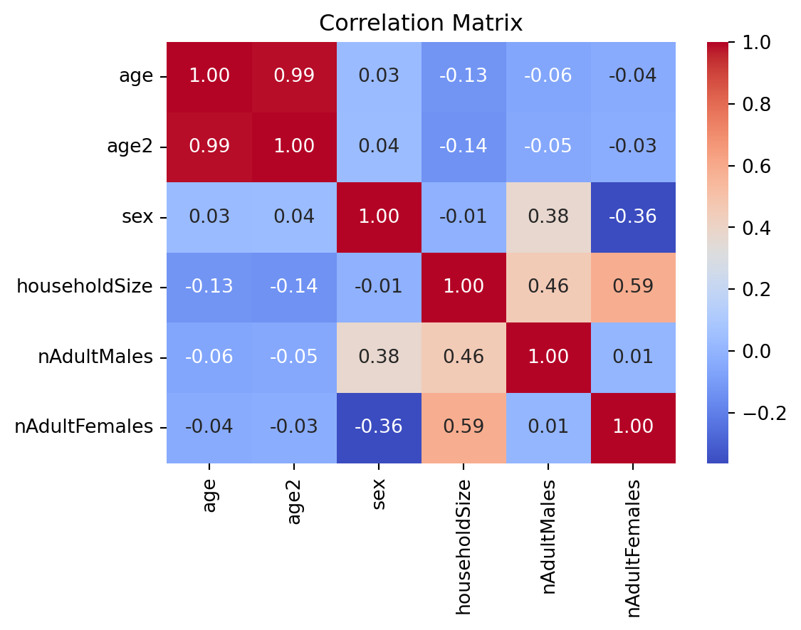
The variables \(age\) and \(age^2\) are strongly correlated, indicating multicollinearity might be an issue. Although, the correlation is lower, the issue may also be present among variables \(houeholdSize\), \(nAdultMales\), and \(nAdultFemales\).
It is then useful to compute statistics to detect or determine the severity of multicollinearity. The most common statistic is the variance inflation factor (VIF): \[ VIF_i = \frac{1}{1-R^2_j} \]
If we had the choice, we would like \(VIF_j\) to be small (other things equal). An arbitrary cutoff value of the VIF often used to conclude multicollinearity is a “problem” is 10 [if VIFj is above 10 — equivalently, \(R^2_j\) is above 0.9].
from statsmodels.stats.outliers_influence import variance_inflation_factor as vif

# Define the independent variables (excluding the dependent variable)
Z = data[['age', 'age2', 'sex', 'householdSize', 'nAdultMales', 'nAdultFemales']]

# Compute VIF for each variable
vif_data = pd.DataFrame()
vif_data["Variable"] = Z.columns
vif_data["VIF"] = [vif(Z.values, i) for i in range(Z.shape[1])]

# Display VIF results
print(vif_data)
Variable VIF
0 age 39.722214
1 age2 22.655474
2 sex 2.769698
3 householdSize 11.785169
4 nAdultMales 5.273431
5 nAdultFemales 6.772311Drop \(houeholdSize\), but keep \(age^2\) beacuse it is needed to capture the nonlinear relationship between age and income.
Z = data[['age', 'age2', 'sex', 'nAdultMales', 'nAdultFemales']]
Y = data['income']  # Dependent variable
Z = sm.add_constant(Z)  # Add an intercept term

mrm = sm.OLS(Y, Z).fit()
print(mrm.summary())
OLS Regression Results
==============================================================================
Dep. Variable: income R-squared: 0.069
Model: OLS Adj. R-squared: 0.063
Method: Least Squares F-statistic: 11.10
Date: Thu, 23 Apr 2026 Prob (F-statistic): 2.50e-10
Time: 15:25:13 Log-Likelihood: -2435.5
No. Observations: 751 AIC: 4883.
Df Residuals: 745 BIC: 4911.
Df Model: 5
Covariance Type: nonrobust
=================================================================================
coef std err t P>|t| [0.025 0.975]
---------------------------------------------------------------------------------
const 2.9583 2.500 1.183 0.237 -1.949 7.866
age 0.4407 0.121 3.646 0.000 0.203 0.678
age2 -0.0046 0.001 -3.209 0.001 -0.007 -0.002
sex 1.6915 0.534 3.166 0.002 0.642 2.741
nAdultMales -1.4387 0.327 -4.406 0.000 -2.080 -0.798
nAdultFemales -0.4803 0.303 -1.584 0.114 -1.076 0.115
==============================================================================
Omnibus: 156.879 Durbin-Watson: 1.955
Prob(Omnibus): 0.000 Jarque-Bera (JB): 286.602
Skew: 1.236 Prob(JB): 5.82e-63
Kurtosis: 4.746 Cond. No. 2.04e+04
==============================================================================
Notes:
[1] Standard Errors assume that the covariance matrix of the errors is correctly specified.
[2] The condition number is large, 2.04e+04. This might indicate that there are
strong multicollinearity or other numerical problems.3.2 Homoskedasticity
Heteroskedasticity occurs when the variance of the error terms (\(u_i\)) is not constant across observations. This violates Assumption 5 of the Ordinary Least Squares (OLS) regression model:
\[ Var(u|x_1,x_2,\dots,x_k) = \sigma^2 \].
In the income regression, heteroskedasticity might occur if, for example, income variability is much higher for high-income individuals than for low-income individuals.
why is it a problem?
OLS estimates are still unbiased [the expected value of the sampling distribution of the estimators is equal the true population parameter value], and consistent [as the sample size increases, the estimates converge to the true population parameter], but the standard errors are incorrect.
Heteroskedasticity invalidates variance formulas for OLS estimators
OLS is no longer the best linear unbiased estimator (BLUE).
The t-tests and F-tests become unreliable, leading to wrong conclusions.
Confidence intervals become misleading, as they might be too narrow or too wide.
3.2.1 Detect Heteroskedasticity
Plot the residuals against the fitted values of the regression. This allows you to visually identify heteroskedasticity if there is an evident pattern in the plot.
If residuals are evenly spread across fitted values \(\rightarrow\) Homoskedasticity.
If widening or narrowing, suggests non-constant variance \(\rightarrow\) Heteroskedasticity.
fitted_values = mrm.fittedvalues  # Predicted Y values from the model
residuals = mrm.resid             # Model residuals

# Scatter plot of residuals vs fitted values
plt.figure(figsize=(7, 5))
sns.scatterplot(x=fitted_values, y=residuals, alpha=0.6)
plt.axhline(0, color='red', linestyle='dashed')  # Reference line at 0
plt.xlabel("Fitted Values of Income")
plt.ylabel("Residuals")
plt.title("Residuals vs. Fitted Values (Heteroskedasticity)")
plt.show()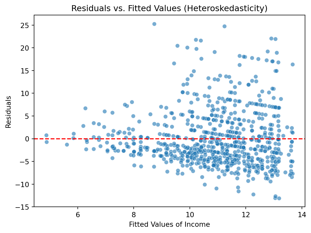
The plot shows geater variation of the residuals at higher levels of income. Heteroskedasticity appears to be an issue in this example.
We could also use formal tests:
The Breush-Pagan test
Departing from a homoskedastic null hypothesis:
\[ H_0: Var(u|x_1, x_2, \cdots, x_k)= Var(u|\boldsymbol{x})=\sigma^2 \] By definition \(Var(u|\boldsymbol{x}) = E(u^2|\boldsymbol{x})-[E(u|\boldsymbol{x})]^2=E(u^2)=\sigma^2\). That is, under the null hypothesis, the mean of \(u^2\) must not vary with \(x_1, x_2, \cdots, x_k\).
Estimate the model:
\[ \hat{u}^2 = \delta_0 + \delta_1 x_1 + \delta_2 x_2 + \delta_3 x_3 + \cdots + \delta_k x_k + \epsilon \]
and test:
\[ Ho: \delta_1 = \delta_2 = \cdots = \delta_k = 0 \]
A large F-statistic or small p-value is evidence agains the null, therefore heteroskedasticity would be detected.
residuals2 = mrm.resid**2
Z = data[['age', 'age2', 'sex', 'nAdultMales', 'nAdultFemales']]
Z = sm.add_constant(Z)  # Add an intercept term

bp = sm.OLS(residuals2, Z).fit()
print(bp.summary())
OLS Regression Results
==============================================================================
Dep. Variable: y R-squared: 0.029
Model: OLS Adj. R-squared: 0.023
Method: Least Squares F-statistic: 4.465
Date: Thu, 23 Apr 2026 Prob (F-statistic): 0.000514
Time: 15:25:13 Log-Likelihood: -4290.3
No. Observations: 751 AIC: 8593.
Df Residuals: 745 BIC: 8620.
Df Model: 5
Covariance Type: nonrobust
=================================================================================
coef std err t P>|t| [0.025 0.975]
---------------------------------------------------------------------------------
const 12.4981 29.546 0.423 0.672 -45.506 70.502
age 1.4149 1.429 0.990 0.322 -1.390 4.219
age2 -0.0083 0.017 -0.488 0.626 -0.042 0.025
sex 4.9734 6.315 0.788 0.431 -7.425 17.372
nAdultMales -10.8536 3.859 -2.812 0.005 -18.430 -3.277
nAdultFemales -3.4987 3.584 -0.976 0.329 -10.535 3.538
==============================================================================
Omnibus: 682.775 Durbin-Watson: 1.978
Prob(Omnibus): 0.000 Jarque-Bera (JB): 17147.833
Skew: 4.211 Prob(JB): 0.00
Kurtosis: 24.842 Cond. No. 2.04e+04
==============================================================================
Notes:
[1] Standard Errors assume that the covariance matrix of the errors is correctly specified.
[2] The condition number is large, 2.04e+04. This might indicate that there are
strong multicollinearity or other numerical problems.Alternatively:
from statsmodels.stats.diagnostic import het_breuschpagan

bp_test = het_breuschpagan(residuals, Z)
bp_stat, bp_pvalue = bp_test[0], bp_test[1]

print(f"Breusch-Pagan Test Statistic: {bp_stat:.4f}")
print(f"P-value: {bp_pvalue:.4f}")

# Implement the Decision Rule:
alpha = 0.05
if bp_pvalue < alpha:
    print("Heteroskedasticity detected (Reject H0)")
else:
    print("No statistical evidence of heteroskedasticity (Fail to reject H0)")
Breusch-Pagan Test Statistic: 21.8495
P-value: 0.0006
Heteroskedasticity detected (Reject H0)White test
Regress \(u^2\) against all explanatory variables, their squares, and interactions. For \(k=2\):
\[ \hat{u}^2 = \delta_0 + \delta_1x_1 + \delta_2x_2 + \delta_{3}x_1^2 + \delta_{4}x_2^2 + \delta_5x_1x_2 +\epsilon \] The null hypothesis: \[ H_0: \delta_1 = \delta_2 = \cdots = \delta_5=0 \]
The White test detects more general deviations from heteroskedasticity than the Breush-Pagan test. A disadvantage is it includes a large number of estimated parameters.
Alternative form of the White test for heteroskedasticity:
\[ u^2 = \delta_0 + \delta_1\hat{y} + \delta_2\hat{y}^2+\epsilon \] Indirectly tests the dependence of the squared residuals on the explanatory variables, their squares, and interactions (contained in \(\hat{y}\) and \(\hat{y}^2\)).
from statsmodels.stats.diagnostic import het_white

white_test = het_white(residuals, Z)
white_stat, white_pvalue = white_test[0], white_test[1]

print(f"White Test Statistic: {white_stat:.4f}")
print(f"P-value: {white_pvalue:.4f}")

# Implement the Decision Rule
alpha = 0.05
if white_pvalue < alpha:
    print("Heteroskedasticity detected (Reject H0)")
else:
    print("No statistical evidence of heteroskedasticity (Fail to reject H0)")
White Test Statistic: 39.6505
P-value: 0.0023
Heteroskedasticity detected (Reject H0)3.2.2 Correct Heteroskedasticity
Remember: If heteroskedasticity is detected, OLS estimates remain unbiased, but standard errors are wrong. We can fix this by using robust standard errors. Several methods (HC0, HC1, HC2, HC3) that differ in how they adjusts for heteroskedasticity and small-sample bias available:
# HC0 (large sample size)

mrm_robust0 = mrm.get_robustcov_results(cov_type="HC0")
print(mrm_robust0.summary())
OLS Regression Results
==============================================================================
Dep. Variable: income R-squared: 0.069
Model: OLS Adj. R-squared: 0.063
Method: Least Squares F-statistic: 14.95
Date: Thu, 23 Apr 2026 Prob (F-statistic): 5.31e-14
Time: 15:25:13 Log-Likelihood: -2435.5
No. Observations: 751 AIC: 4883.
Df Residuals: 745 BIC: 4911.
Df Model: 5
Covariance Type: HC0
=================================================================================
coef std err t P>|t| [0.025 0.975]
---------------------------------------------------------------------------------
const 2.9583 2.578 1.147 0.252 -2.103 8.019
age 0.4407 0.135 3.276 0.001 0.177 0.705
age2 -0.0046 0.002 -2.695 0.007 -0.008 -0.001
sex 1.6915 0.519 3.257 0.001 0.672 2.711
nAdultMales -1.4387 0.299 -4.816 0.000 -2.025 -0.852
nAdultFemales -0.4803 0.265 -1.816 0.070 -1.000 0.039
==============================================================================
Omnibus: 156.879 Durbin-Watson: 1.955
Prob(Omnibus): 0.000 Jarque-Bera (JB): 286.602
Skew: 1.236 Prob(JB): 5.82e-63
Kurtosis: 4.746 Cond. No. 2.04e+04
==============================================================================
Notes:
[1] Standard Errors are heteroscedasticity robust (HC0)
[2] The condition number is large, 2.04e+04. This might indicate that there are
strong multicollinearity or other numerical problems.Other options:
# HC1 (Stata default, recommended for small/moderate samples)
mrm_robust1 = mrm.get_robustcov_results(cov_type="HC1")
# print(mrm_robust.summary())

# HC2 (Adjusts for leverage points)
mrm_robust2 = mrm.get_robustcov_results(cov_type="HC2")
# print(mrm_robust_HC2.summary())

# HC3 (More conservative, useful for small samples)
mrm_robust3 = mrm.get_robustcov_results(cov_type="HC3")
# print(mrm_robust_HC3.summary())
3.3 Serial correlation
Autocorrelation, also known as serial correlation, occurs when the error terms (\(u_i\)) are correlated across observations. It emerges when observations are spatially or logically related (e.g., geographic clustering), if the residuals from one observation are correlated with another, this suggests systematic patterns that OLS fails to capture. This violates assumption 6, that the error terms should be independently distributed:
\[ E(u_i,u_j) = 0, \ \ \ for \ \ i \ne j \]
why is it a problem?
Even though OLS estimates remain unbiased:
Standard Errors are underestimated, making t-tests and confidence intervals invalid.
t-statistics and F-statistics become inflated, leading to a higher probability of Type I errors (rejecting a true null hypothesis).
OLS is no longer the Best Linear Unbiased Estimator (BLUE)
3.3.1 Detect Autocorrelation
Autocorrelation is a serious issue in time series data where observations are sequential (e.g., stock prices, GDP growth, inflation, interest rates) as the residuals from one period maybe corelated with the next period. If the data is a time series one simple way to check for autocorrelation is to plot residuals over time. If the residuals appear randomly scattered around zero, there is evidence of no autocorrelation. But if residuals form a clear pattern (e.g., trending up/down) or alternate frequently (high-low-high-low), there is evidence of positive or negative autocorrelation, respectively.
Durbin-Watson Test
The Durbin-Watson (DW) test is primarily used for time series data, where observations are sequentially ordered over time. It detects first-order autocorrelation in the residuals of a regression model, meaning that the error at time \(t\) depends on the error at time \(t−1\).
The null hypothesis \(H_0\) states that there is no autocorrelation in the residuals:
\[ H_0: \rho = 0 \] The Durbin-Watson statistic, \(DW\), is computed as: \[ DW = \frac{\sum_{t=2}^n(u_t-u_{t-1})^2}{\sum_{t=1}^n u_t^2} \]
It measures the sum of squared differences between adjacent residuals relative to the total sum of squared residuals.
\(DW \approx 0:\) Strong positive autocorrelation.
\(DW \approx 4:\) Strong negative autocorrelation.
\(DW \approx 2:\) No autocorrelation.
from statsmodels.stats.stattools import durbin_watson

# Compute Durbin-Watson statistic
dw_stat = durbin_watson(residuals)
print(f"Durbin-Watson Statistic: {dw_stat:.4f}")
Durbin-Watson Statistic: 1.9551A disadvantage of the DW test is that it only detecs autocorrelation of first-order. For higher-order Autocorrelation use the Breusch-Godfrey Test.
Breusch-Godfrey Test
The Breusch-Godfrey test can detect autocorrelation of any order (\(p\)), meaning it checks if the residual at time \(t\) is related to residuals from previous periods \((t−1,t−2,...,t−p)\).
The test examines whether the residuals exhibit serial correlation:
\[ H_0: \text{No autocorrelation} \]
The null hypothesis states that residuals are not autocorrelated, that is, no serial correlation (errors are independent).
from statsmodels.stats.diagnostic import acorr_breusch_godfrey

# Specify the bumber of lags
bg_test = acorr_breusch_godfrey(mrm, nlags=2)
bg_stat, bg_pvalue = bg_test[0], bg_test[1]

print(f"Breusch-Godfrey Test Statistic: {bg_stat:.4f}")
print(f"P-value: {bg_pvalue:.4f}")

# Implement the decision Rule
alpha = 0.05
if bg_pvalue < alpha:
    print("Autocorrelation detected (Reject H0)")
else:
    print("No evidence of autocorrelation (Fail to reject H0)")
Breusch-Godfrey Test Statistic: 0.5242
P-value: 0.7694
No evidence of autocorrelation (Fail to reject H0)The tests indicates that the residuals in our model are not serially correlated.
3.3.2 Correct autocorrelation
If autocorrelation is detected, we need to adjust our regression model to obtain valid inference. Although not necessary in our model, some solutions can be implemented in python as follows:
Newey-West Robust Standard Errors
Re-estimate model with Newey-West robust standard errors to correct t-tests and confidence intervals for autocorrelation. It allows for autocorrelation up to lag 2.
mrm_newey = mrm.get_robustcov_results(cov_type="HAC", maxlags=2)

# Display results
print(mrm_newey.summary())
OLS Regression Results
==============================================================================
Dep. Variable: income R-squared: 0.069
Model: OLS Adj. R-squared: 0.063
Method: Least Squares F-statistic: 15.49
Date: Thu, 23 Apr 2026 Prob (F-statistic): 1.63e-14
Time: 15:25:13 Log-Likelihood: -2435.5
No. Observations: 751 AIC: 4883.
Df Residuals: 745 BIC: 4911.
Df Model: 5
Covariance Type: HAC
=================================================================================
coef std err t P>|t| [0.025 0.975]
---------------------------------------------------------------------------------
const 2.9583 2.516 1.176 0.240 -1.981 7.898
age 0.4407 0.133 3.301 0.001 0.179 0.703
age2 -0.0046 0.002 -2.684 0.007 -0.008 -0.001
sex 1.6915 0.502 3.368 0.001 0.706 2.677
nAdultMales -1.4387 0.303 -4.753 0.000 -2.033 -0.844
nAdultFemales -0.4803 0.246 -1.956 0.051 -0.962 0.002
==============================================================================
Omnibus: 156.879 Durbin-Watson: 1.955
Prob(Omnibus): 0.000 Jarque-Bera (JB): 286.602
Skew: 1.236 Prob(JB): 5.82e-63
Kurtosis: 4.746 Cond. No. 2.04e+04
==============================================================================
Notes:
[1] Standard Errors are heteroscedasticity and autocorrelation robust (HAC) using 2 lags and without small sample correction
[2] The condition number is large, 2.04e+04. This might indicate that there are
strong multicollinearity or other numerical problems.The HAC (Heteroskedasticity and Autocorrelation Consistent) covariance estimator corrects standard errors to account for both issues.
Generalized Least Squares (GLS)
GLS adjusts for autocorrelation by modeling error terms as an AR(1) process, that is,
\[ u_t = \rho u_{t-1} + \epsilon \]
# Fit GLS model (assumes AR(1) error structure)
mrm_gls = sm.GLSAR(Y, Z, rho=1).iterative_fit()

# Display results
print(mrm_gls.summary())
GLSAR Regression Results
==============================================================================
Dep. Variable: income R-squared: 0.069
Model: GLSAR Adj. R-squared: 0.063
Method: Least Squares F-statistic: 11.01
Date: Thu, 23 Apr 2026 Prob (F-statistic): 3.03e-10
Time: 15:25:13 Log-Likelihood: -2432.5
No. Observations: 750 AIC: 4877.
Df Residuals: 744 BIC: 4905.
Df Model: 5
Covariance Type: nonrobust
=================================================================================
coef std err t P>|t| [0.025 0.975]
---------------------------------------------------------------------------------
const 3.1093 2.503 1.242 0.215 -1.804 8.023
age 0.4335 0.121 3.583 0.000 0.196 0.671
age2 -0.0046 0.001 -3.149 0.002 -0.007 -0.002
sex 1.6946 0.535 3.165 0.002 0.644 2.746
nAdultMales -1.4362 0.327 -4.393 0.000 -2.078 -0.794
nAdultFemales -0.4940 0.303 -1.630 0.104 -1.089 0.101
==============================================================================
Omnibus: 158.283 Durbin-Watson: 1.994
Prob(Omnibus): 0.000 Jarque-Bera (JB): 291.453
Skew: 1.243 Prob(JB): 5.15e-64
Kurtosis: 4.773 Cond. No. 2.01e+04
==============================================================================
Notes:
[1] Standard Errors assume that the covariance matrix of the errors is correctly specified.
[2] The condition number is large, 2.01e+04. This might indicate that there are
strong multicollinearity or other numerical problems.Important:
When the nature of the data is time-dependent, autocorrelation might be strong and persistent. In such cases using proper econometric time series techniques would be more appropriate than simply trying to correct the issue within the OLS framework.